Assessing the Quality of Soundings
Ensuring that your hydrographic data complies with the latest standards can be difficult, particularly as standards continually change with new advances in technology. Simon Squibb discusses a ‘binning’ technique that may improve data confidence for surveyors and clients.
The standards for hydrographic measurements are regularly reviewed to cope with advances in technology and the demand for higher accuracy data, which continually increases. For example, last year the 4th edition of the international standard, IHO S44 (1), was modified by various hydrographic authorities to meet wider application.
To aid their surveyors in assessing the quality of data collected, Andrews Survey has developed a post-processing package, PP2000: a set of tools to give surveyors and clients alike a greater degree of confidence in the validity of their data. In common with other survey post-processing packages, PP2000 includes tools for data cleaning, smoothing, tidal reduction etc. For the purposes of this paper, only the assessment of the quality of the final dataset, after all other processes are complete, will be considered.
The software has been successfully tested on datasets in excess of 500,000 data points. To date it has only been used with single beam datasets. However, there is no reason why the techniques described here cannot be applied to multibeam data.
How to Assess Sounding Data?
After a survey has been completed and the data cleaned to remove accidental errors and the effect of tide, the quality of the data may then be checked by assessing the repeatability of the measurements, looking at tie points on cross lines. The surveyor could plot the data at a scale sufficient to check each tie by eye. However, even for a small survey this would require some data thinning and it is time-consuming and subject to the surveyor’s experience and understanding.
The method employed here is to use a ‘binning’ process. The data is read into a user-defined cell matrix, each cell or bin holding the reference to any data that falls geographically within it. The user may view the data as a colour-coded, cell-averaged map showing the trend within the dataset. Any major problems are then highlighted by colour mismatch.
Alternatively, the difference between the maximum and minimum of the data within each cell can be shown. This method will highlight not just miss-ties on tie lines but any outliers occurring along the lines.
The cell size used when mapping the data will have a significant effect on the maximum and minimum values held in each cell, particularly in areas of high rates of change, for example in sand-wave fields. Figure 1 shows two views of the same line crossing and the same colour exaggeration. In the first, the data has been binned using a cell size of 5 metres; the second at 2 metres. The orange cells show a difference of 0.6 - 0.8 metres and the green less than 0.1 metre. The user can list the data held within an individual cell to check whether observed differences are real or caused by erroneous data missed in the data cleaning process. Because the binning process is highly dependent on computer memory, to cope with large datasets the user can choose subsets from the main dataset and map them at a much finer cell size.
Obviously, to check every line crossing in the manner described is time-consuming and cumbersome. An overall measure of its consistency can be calculated more rapidly by looking statistically at the tie points within the dataset. The difference in the line average from within each bin containing data for more than one survey line is calculated. It is then graphed to show the frequency distribution of differences. Similarly, the nearest neighbour from each line is also detected from within these cells and the difference calculated. Given enough tie points within the dataset, the results may be analysed statistically to give an overall measure of the consistency of the dataset.
There is also a facility for detecting whether line data in the cell cross. If this option is selected, only crossing datasets are used in the average data statistics. The following examples show how this helps in assessing whether the survey has reached the required standard.
Actual Examples
Example 1 Assessing Data Consistency
Andrews Survey conducted the survey depicted in Figure 2 over a four hour period, about five nautical miles from a port tide gauge, using a single beam echosounder, DGPS for positioning and an SV probe for speed of sound. A heave compensator was not used and maximum heave observed was less than 1 metre. The average depth at the survey site is 39 metres, with a depth range of 4 metres. The tidal range is 1.9m at springs.
The error budget calculated for this survey is shown in Table 1.
The error budget was calculated using methods described in Hydrographic Department Professional Paper 25, The Assessment of the Precision of Soundings (2). Comparing data from within the same dataset, certain errors are going to remain constant and thus cannot be used to assess the consistency of the survey. Errors (a) to (e) would be fixed or negligible for this survey. This leaves a theoretical maximum error of 0.39m for the survey. The survey was actually conducted over a single high-water period with a maximum tidal variation of 0.3m. As the major factor influencing the error budget (and thus the cross line statistics) is the co-tidal correction, the maximum error for the tides was re-calculated to 0.15m. This gives a new theoretical maximum of 0.31m for the survey.
The international standard for confidence level is 95 per cent or two standard deviations away from the mean. Thus, if we analyse the data collected in the manner described above, 95 per cent of the differences observed on the ties should fall below 0.31 metres. The following graphs depict what was found in practice. The statistics were calculated with the tolerance for nearest neighbour detection set at 0.5 metres and line crossing detection switched on. Figure 3 shows two QC plots available to the operator. The first shows a histogram depicting the averaged and nearest neighbour frequency distribution; the second shows the observed miss ties plotted against depth under the target standard.
The calculated average and standard deviation are within expectations, with the averaged values showing a mean of 0.09 and standard deviation of 0.08. This gives a 95 per cent confidence level of 0.25, based on 83 crossings. The 95 per cent confidence level for the nearest neighbour data was 0.24, based on 103 tie points. The average distance apart for the nearest neighbour is 0.17m, with a standard deviation of 0.12m.
The plot of the observed differences is based on the averaged data and gives an indication as to how well the dataset adheres to the chosen standard. This is not the whole story, however, as line spacing, data coverage, positioning etc. have not been taken into consideration. Nevertheless, it does provide useful information on the consistency of the data.
Example 2 Assessing Improvements in Data Quality
The survey depicted in Figure 4 was a larger regional survey, conducted over two days in an area of sand-waves. Again, a single beam echo-sounder was employed, DGPS for positioning and an SV probe for speed of sound. No heave compensator was used and maximum heave observed was less than 1 metre. The data was reduced using predicted tides from the nearest standard port, fifty nautical miles from site, and co-tidal corrections from a co-tidal and co-range chart. The mean spring tidal range on site varied between 3.8 and 3.4 metres, compared with 4.4 metres at the standard port.
The stripes on the Northeast - Southwest lines are sand-waves up to 5 metres high.
The worst case error budget for this survey is shown in Table 2.
If errors (a) to (e) are ignored, then the expected error is reduced to 0.63m. For purposes of analysis the data was binned at a cell size of 5m. Line crossing detection was switched off and the nearest neighbour tolerance was set to 0.75 metres. The results show that the calculated average and standard deviation do not fall within expectations. The averaged values show a mean of 0.35 and a standard deviation of 0.25, giving a 95 per cent confidence level of 0.85, based on 55 ties. The 95 per cent confidence level for the nearest neighbour was slightly better, at 0.76, based on 38 tie points. The average distance apart for the nearest neighbour is 0.35m, with a standard deviation of 0.17m.
There were a significant number of outliers caused by the large sand-waves found in the area. By decreasing the cell size to 3 metres it was possible to bring the 95 per cent confidence level for the averaged values in line with that calculated for the nearest neighbour, as shown in Figure 5.
The most significant errors affecting the data are those associated with the tidal reduction and were probably underestimated in the initial error budget for the survey. Due to the size of the survey area, a significant improvement was seen when co-tidal factors were interpolated for each point, as opposed to the site-centred factors used above. Figure 6 shows that after re-interpolation of the tides the 95 per cent confidence level was reduced to 0.54m.
Conclusion
Using a simple statistical test on the tie points from a sounding survey it is possible to assess the consistency of a dataset and thus the overall quality of the survey, particularly of the tidal reduction. This is not to say that the survey as a whole has achieved any particular standard but a good indication is given that expected errors have been reduced to a minimum.
The Andrews Survey software gives the user a tool that allows swift analysis of the dataset and efficient isolation of potential problem areas, thus giving both client and surveyor greater confidence in the validity of the data.
Although the software has only been used with single beam datasets, there is no reason why the same procedure cannot be used to produce similar results with any XYZ dataset, including multibeam data.
References
- Wells, D.E. and Monahan, D. IHO S44 Standards for Hydrographic Surveys and the Variety of Requirements for Bathymetric Data. The Hydrographic Journal, Issue 104, April 2002. Available online at www.hydrographicsociety.org
- Hydrographic Department Professional Paper No.25, The Assessment of the Precision of Soun-dings. Hydrographic Department 1990
Bibliography
- International Hydrographic Organisation, 1998. IHO Standards for Hydrographic Surveys, International Hydrographic Organisation Special publication No 44, 3rd edition
- Hydrographer of The Navy, General Instructions for Hydrographic Surveyors, Seventeenth Edition. Hydrographer of the Navy 1996

Value staying current with hydrography?
Stay on the map with our expertly curated newsletters.
We provide educational insights, industry updates, and inspiring stories from the world of hydrography to help you learn, grow, and navigate your field with confidence. Don't miss out - subscribe today and ensure you're always informed, educated, and inspired by the latest in hydrographic technology and research.
Choose your newsletter(s)