Handling Sonar Data from AUV Operations

During the past few years, autonomous underwater vehicles (AUVs) have established a greater presence in the hydrographic survey market and in the collection of oceanographic environmental data. These vehicles can transit non-stop for long periods of time, and can work in areas in which traditional survey vessels are not very effective. Though the cost can be justified over time, making AUVs economical for the amount of work done, limitations occur in handling the data from these vehicles. How do we effectively and efficiently go from vehicle to final product?

By Harold Orlinsky and Judy Bragg.

Offloading Data From the AUV

A tremendous amount of bathymetry and side scan data is collected during each mission. In a 4-hour transect, 70GB may be collected, which can take more than an hour to download via a USB link. A removable hard drive may not practical as the AUV need to maintain the watertight integrity, so time is always allocated for this step. On some larger AUVs, entire sections of the fish containing the batteries and data storage are removed.

Preprocessing Format Conversion

Once the data is offloaded, the sensor data must be in a usable format for processing.  Making it a common format to industry standards, such as HSX, GSF or XTF, will allow more software applications to handle the data.

Throughout this article, all files are converted to the HYPACK HSX format and processed using HYPACK® software: MBMAX64 for bathymetry and HYSCAN for side scan processing.

Data from some interferometry systems on board AUVs have an additional step, and must be processed to a data format before the conversion to the HYPACK® HSX format.  Other sonar data can be converted directly to the HSX format.

For efficiency during the survey mission, these data conversions can be done on board the AUV. After each line of data is collected, the raw files can be converted to the processing format while still on board the vehicle. We still have to account for the time required to unload the data from a vehicle, but we can then immediately begin work in the processing programs.

Errors

Each sensor on the AUV can contribute some degree of depth or position error. Three that have been seen are navigation drift and adjustments to the data, sonar update rate versus rate of turn, and AUV depth calculations (pressure sensor) and potential errors.

Navigation Adjustments

The navigation of the AUV is not as precise as systems onboard vessels, as the vehicles relay on DVLs and INS for position. On some vehicles, these sensors track very well; on others, position drift is significant. Data processing software has tools to help clean the data:

• Merge a processed navigation file into the sonar data. The navigation file is one that has been adjusted to account for vehicle drift and provides the best estimate of the true position for the AUV. The original navigation file – extracted from the vehicle and then corrected with known markers on the seafloor, to create an enhanced navigation file. During the conversion, this file replaces any navigation recorded during the mission.  
• Adjust the position with a known offset – a value determined at the end of a line – scaled to the distance travelled along the lines. Prior to a dive, the AUV obtains a GPS fix. At the completion of the line, the AUV obtains a new fix. The difference of the GPS position and the AUV positions can be used to adjust the line. Although not exact, as this method assumes a constant drift and speed throughout the line, the adjustment is scaled to the distance travelled on the survey line. Observing the depth as a profile line, we can see this shift makes a noticeable depth difference at the end of the line.

Coverage on Turns in the Survey Line

The second area of error can be observed during a turn in the mission. Ideally, all lines are designed as a single segment transect. At the end of each segment, a break in the data will occur and a new line will begin once the turn is completed. However, in the example below, the vehicle turns 30 degrees in eight seconds. In most cases, this is not a problem.

During this mission, the multibeam sonar was updating at 2 Hz. It was determined that, with this ping rate, the bottom had full coverage at the vehicle speed (2 knots) and water depth (110 meters); however, the outer portion of the swath (175 meters from nadir) did not completely ensonify the bottom as the distance travelled of the outer beams exceeded the beam footprint size, through a turn of less than 4 degrees per second.

The survey is left with a holiday in this instance. The system would need to ping at a rate greater than 12Hz to fill the area. (A Rate of Turn filter would remove the data completely.)

In shallow water, this would be attainable, but in this case, the mission could replace the bent line with two straight lines that intersect at the turn to completely cover the area. The drawback, of course, is added time to survey the full length of both intersecting lines.

Depth Calculation From the Pressure Sensor

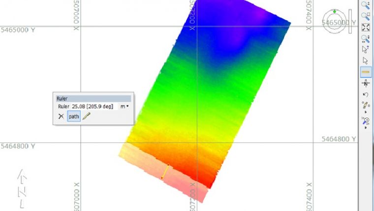
The depths of the AUVs come from pressure sensors. Using the standard formula of UNESCO, we can compute the towfish depth (stored in the HSX files with a DFT identifier) and add it to the sonar values to determine the actual seafloor depth (stored in the HSX files with a DFT identifier) and add it to the sonar values to determine the actual seafloor depth. In Figure 3, notice the dive at the beginning of the line, and the survey data at a constant attitude when no towfish depth is applied.

This calculated depth, however, is not exact. The uncertainty of this sensor is based upon factors that are variable - sea action and wave heights and atmospheric pressure - and measuring them for real-time corrections would be impossible. Waves act as additional water on top of the AUV and change the pressure reading from the onboard sensor. Slightly less error will come from the change of the atmospheric pressure during the mission. We could measure the start and end pressure, and interpolate across the mission time, however, the rate of change may not be constant.

• Uncorrected, the pressure-to-depth curve holds these small errors. Our sample data shows 60 cm peak-to-valley measurements in the pressure reading from a single dive mission.

If we measure the seafloor depth and do not apply any draft correction, we observe a depth variation in the magnitude of 20cm. Using this as a baseline bathymetry, we can try to adjust the pressure sensor depth to provide a depth correction to the AUV without modifying the seafloor topography.

• Applying the depth from the pressure sensor directly, we can immediately observe high frequency jitter throughout and a peak-to-valley measurement of 55cm.
• Applying a 5 second averaging to the depths, both the high and low frequency jitter is removed, and the peak-to-valley depth is less than 23 cm, in alignment of the baseline seafloor depth.

Conclusion

AUVs will increase their presence in the market for survey and oceanographic work. But, like all sensors, they are not without errors. Depth and position errors from AUVs can be attributed to the payload, vehicle size and environmental conditions.  This article presents a few issues that you may encounter using these vehicles.  Some may be easier to fix; simply designing a mission with only straight lines, would be beneficial (if practical during the survey). And some – navigation drift, and error introduced by wave action – can only be estimated, so the adjusted data may not be exactly accurate.