Improving the Accuracy of ADCP Discharge ­Measurements

There is a key new feature in the discharge measurement software ViSea DAS that allows the user to add a bottom profile. By doing so, side extrapolation from the start and end points of the survey track to the shore is calculated automatically using dGPS positioning. This removes the error inherent in estimating the track to shore distance for each individual track, which is the current method used in comparable software packages. This paper describes research that validates this new approach.

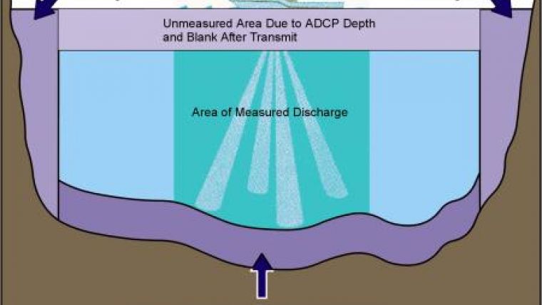
Discharge measurements are important for the characterisation of rivers and are the basis of many models. There are many methods to measure discharge, all of which are limited to the measurement area (­Valentin, Kölling 1995). This excludes the top, bottom and nearshore areas of the profile (Figure 1). The top of the water column is extrapolated in the software by specifying the ADCP depth and calculating the blanking zone. The bottom of the water column, approximately 6%, though measured, is excluded due to interference from side-lobes, is also extrapolated by the software. The nearshore areas, being too shallow to survey, are unmeasured, leaving the surveyor to estimate the distance from the vessel to the shore. This distance is entered to calculate the total river width and the nearshore discharge.

As the true bottom profile is unknown, the software contains various extrapolation options to calculate the nearshore discharge. The estimation of both the bottom profile type and the distance to shore introduces errors into the discharge measurement.

Measurement System

One standard method to measure discharge makes use of ADCPs (Acoustic Doppler Current Profilers). ADCPs calculate current speed and direction based on the measurement of the Doppler Effect. They have four ultrasound transducers that function both as transmitters and receivers. During a measurement, an ADCP is mounted on a survey vessel (Figure 2), with the transducers facing downwards. A sound pulse is transmitted that reflects off particles in the water. Change in relative distance between the ADCP and the particles causes a Doppler shift, whereby the frequency of the sound waves change. When the reflected sound wave returns to the transducers, the frequency shift is measured and used to calculate the relative velocity between the ADCP and the particles in the water (RD Instruments 1996).

A discharge measurement is based on the average of a minimum of ten transects from shore to shore.

A combination of GNSS with RTK (real-time kinetic) coverage and accuracy and a motion sensor is used to ensure accurate measurements. The motion sensor is used to compensate the vessel’s motion for roll, pitch and heave and heading. These are used to obtain accurately positioned depths, when the positioning antenna and the transducer are not on the same vertical axis.

Standard Method

For the standard method, the surveyor estimates the nearshore distance at the start and end of each transect and enters these values into the software program. This estimation of the nearshore distance introduces an error as the surveyor must estimate the distance visually and repeat the exercise for each transect. As such, the river width will vary for each transect. The use of laser range finders was discarded due to operational difficulties. To minimise this source of error, the previous version of ViSea DAS allowed the user to insert waypoints. In this case, the surveyor estimates the distance once at the beginning of the measurement and the software uses these waypoints to calculate the discharge for all the following transects.

Of course, in this case the bottom geometry is still an unknown. The software allows a choice between triangular, square and user-specified coefficients, to determine how the flow area is calculated. However, this remains an estimate.

Improved Method

ViSea DAS automatically determines the points on the shore as a function of the measured coordinates and altitude from the GPS. The bottom geometry is no longer estimated but measured in two steps: 1. during low water level conditions (in the summer months) the nearshore profile is measured with land measurements 2. during high water level conditions (in the winter months) the deepwater profile is measured with a vessel mounted ADCP. The combination of these two measurements gives a full bottom profile. This profile (coordinates and altitude) is then imported into the Survey Toolbox (Figure 3). It calculates the additional nearshore discharge from side extrapolation between transect start/end point and shoreline waypoints. This removes the inherent error in estimating the track to shore distance for each individual track, because the software uses the same shoreline waypoint for the calculation of the nearshore discharge for all tracks. Additionally, the bottom geometry no longer needs to be estimated.

Case Study

A test measurement was used to compare the calculated discharge values using the previous version of the software, where the nearshore distance at each transect is estimated by the surveyor at the beginning and end of a transect, and the new version of the software. In this version, the software automatically chooses the right points on the shore from an implemented bottom profile based on the measured coordinates and altitude from the GPS. The test period included discharges ranging from 350 to 400m³s^-1.

A comparison of the discharge values of the measured area including the top and bottom area from these two software versions shows no significant difference using the bottom track as reference. In our example, the mean relative difference is just -0.19%.

The comparison of the total discharge shows a mean relative difference of 0.35% using the bottom track as reference (Figure 4).

The difference between these two analyses lies in the calculated nearshore discharge. In our example, comparison of the calculated nearshore discharge from both software versions shows a difference of 19% using the bottom track as reference (Figure 5). The discharge at the left-hand and right-hand shore varied greatly between the old and the new version of extrapolation.

Table 1: Comparison of the edge distance in the two software versions (estimated in ‘ViSea old’ and calculated in ‘ViSea new’) and the nearshore distances.

Table 1 shows a comparison of the edge distances and nearshore discharges from both software versions. On the left-hand side are the edge distances estimated by the surveyor, in metres, which must be filled in by hand in the ‘old’ version. On the right-hand side are the edge distances calculated automatically by the new feature.

Conclusion

A key new feature in ADCP analysis software automatically chooses the correct shoreline waypoints, delivering more consistent and accurate discharge data. The inherent error in estimating the track to shore distance for each individual track is removed by automatically choosing the shoreline waypoints as a function of measured coordinates and altitude from the GPS. As a result, the determination of the nearshore discharge is improved, ultimately resulting in a more accurate discharge value for the unsurveyable section of a river transect.

More Information

Valentin, F.; Kölling, C. (1995): SIMK-Durchflussmessungen. In: Wasserwirtschaft 85, Heft 10, Seite 494-499.

RD Instruments (1996): Acoustic Doppler Current Profiler – Principles of Operation – A Practical Primer. Second Edition for Broadband ADCPs, San Diego, California.

Simpson, M.R. (2001): Discharge measurements using a broad-band acoustic Doppler current profiler. United States Geological Survey. Sacramento, California.

Ms. Spitzner completed her studies in Physical Geography in 2009, specialising in climatological geography and atmospheric research. She moved from the Federal Environment Agency Germany to Aqua Vision in 2011, where she is responsible for measuring and analysing ADCP and multibeam data.

Ms. Ní Fhlaithearta graduated in Earth Sciences (BSc. Hons), after which she gained an MSc. in Earth Systems Science. She worked as a researcher at the University of Utrecht, specialising in biogeochemistry. She has been working at Aqua Vision as a data analyst since 2010.