Lidar Bathymetry on the Alaskan North Slope

In June 2014, the Bureau of Economic Geology, a research unit at the University of Texas at Austin, was contracted to conduct an airborne bathymetric Lidar survey on the Alaskan North Slope. The purpose of the project was to further determine, understand, and map the local landscape and thaw-lake attributes of an area west of the Dalton Highway and Sagavanirktok (Sag) River, approximately 30km southwest of Deadhorse, Alaska. Researchers from the Bureau had visited the area in 2012 and found bathymetric Light Detection and Ranging (Lidar) to be an effective tool for measuring the area’s lakes. The group returned in July 2014 and conducted numerous flights using the Chiroptera airborne Lidar system manufactured by Airborne Hydrography AB, a Leica company, of Sweden. Read on for more details of the project.

Chiroptera has a near-infrared red wavelength of 1.064µm for topographic (topo) data collection and a green wavelength of 0.515µm for bathymetric (hydro) data collection. The system also encompasses a high-resolution Hasselblad camera that collects natural-colour (RGB) or colour-infrared (CIR) imagery. All of these sensors were used in conjunction to acquire precise 3 D geographic data and supplemented with high-resolution CIR imagery.

The unique Alaskan North Slope micro-topography supports various potential fish habitat water bodies and wetland areas with arctic tundra vegetation. Shallow thaw lakes, less than 2m deep in general, are a major component of the tundra landscape of the Alaskan North Slope, where they compose approximately 20% of the total area. They are completely ice free only a few weeks in a calendar year, so fieldwork was scheduled accordingly, beginning in mid-July. The lakes’ depth, ice growth, and decay determine whether they are suitable habitat for wildlife and aquatic fauna, as well as for industrial development. Winter ice is assumed to be 1.5 to 2m thick in this area, and any liquid water most likely lies below winter ice and talik in the central basins of these lakes if the water is deeper than 2m. Survey findings were particularly important for the project sponsor because they would reveal lakes deeper than 2m, suitable for building ice roads). Findings would also assist other environmental and hydrological assessments in the area.

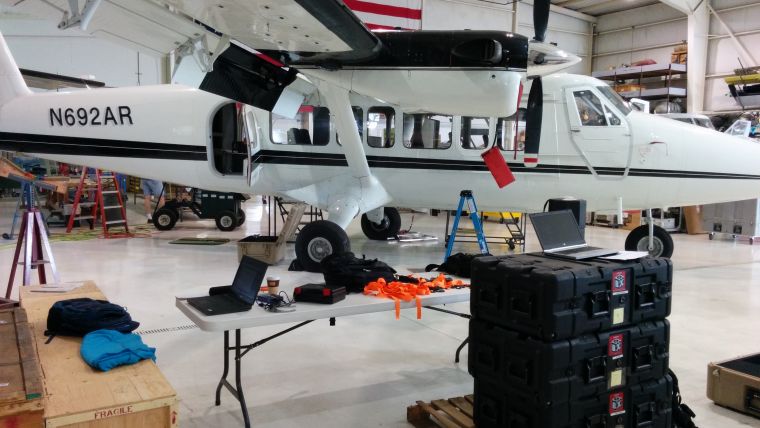
A De Havilland Canada DHC-6 Twin Otter aircraft, along with two pilots and a mechanic, was assigned to the project. Researchers from the Bureau travelled from Austin, Texas, to Grand Junction, Colorado, where the aircraft was staged. Equipment was shipped to the base location at Grand Junction, where system installation and local testing procedures were completed (Figures 1 and 2). Test and calibration flights were completed in Grand Junction to ensure full system functionality before the production phase of the survey began in Alaska.

Survey Set-up

GNSS receivers on the ground were set up at different locations to maximise geometric data quality of the acquired Lidar data. Static geographic positional data acquired from each ground station were differentially corrected by using precise GNSS orbit and clock information. Because of the remote location of the survey area, we used multiple post-processing services and averaged the final solutions to achieve the most acceptable values. Canadian Spatial Reference System (CSRS), University of New Brunswick GAPS, and Trimble CenterPoint RTX provide such services free of charges and turnaround time is generally a few minutes for each 1-hour data file uploaded. In addition to temporary established ground stations, data from two permanent (PU01 and PB0C) Continuously Operating Reference Stations (CORS) were downloaded for confirmation and/or backup purposes. For Lidar system calibration purposes, geodetic level ground-truth data were acquired over the taxiway at Prudhoe Bay Airport using a kinematic dual-frequency GNSS system. For both Lidar scanners, the average vertical offset was measured at less than 1cm, while the standard deviation was calculated at approximately 3cm compared to the points collected at runway pavement. We also examined and corrected any evident Lidar system calibration errors caused mostly by incorrect inertial navigation system (INS) rotation angles of roll, pitch and yaw. These errors can be detected through analysis of adjacent and opposing Lidar strips. In theory, if no rotational misalignments are present, Lidar points registered from different strips should match each other seamlessly on an unobstructed surface; although not expected to have perfection, it is possible to achieve very close results in practice. Calibration procedures were applied to both scanners individually, where average roll and pitch biases were measured to be less than 2.6cm.

Conducting the Survey

A total of 95 lines were flown from north to south and south to north to cover the survey area. The average flight line was approximately 50km long, where laser swath footprint on the ground was calculated to be 280 to 290m wide, flying at 400m altitude from the ground. To compensate for the changing ground elevation (30m in the north, 95m in the south), pilots monitored the atmospheric pressure and adjusted the aircraft altitude to maintain a constant Lidar swath width. Both topo and hydro scanners acquired data simultaneously; the topo scanner emitted light pulses at a speed of 300kHz and recorded discrete pulses (up to 4 returns), compared to the hydro scanner, which acquired data at 35kHz speed and recorded waveform information with 1,024 samples in each shot. The average point density on the ground surface was calculated at 14 points and 1.8 per m2 for each scanner respectively. An average flight line consisted of 33 million points (~1GB) for hydro lines and 220 million points (~7GB) for topo lines. A total of 21 billion points were recorded with the topo scanner, and the hydro scanner registered 3 billion points, for a total of 4 terabytes of raw data.

Leica Lidar Survey Suite LLS v2.09 was used to convert raw data files into industry-standard LAS1.2 and XYZ (ASCII) file formats for output. Because LAS datasets are in binary format, they provide quick and easy access to information, either for analysis or visualisation purposes. Datasets from both scanners were tiled to 1,000 x 1,000m to simplify the computational requirements for data viewing and analysis. As a result, 829 tiles were generated across the survey area, and each tile included a 20m buffer zone in each direction to generate a seamless 1m digital elevation model (DEM) for mapping purposes.
For bathymetric calculations, water bodies shallower than 0.1m and smaller than 1,000m2 in surface area were excluded. The minimum volume calculation was set at 34m3. Every water body was labelled with its latitude and longitude information, in Universal Transverse Mercator (UTM) coordinate format, based on the midpoint determined from the Lidar dataset. Table 1 illustrates two samples where each water body was calculated to include area size, depth, and volume.
Though a dense sampling of bathymetric Lidar returns was captured from the bottom of the water column, a number of larger water bodies (<20) did not have sufficient returns registered from the bottom to have full representation. This deficiency was due to depth, clarity and reflectivity issues in the water column or at the water surface (Figures 3 and 4), possibly caused by suspended materials or aquatic vegetation content. In such scenarios, maximum possible depth was calculated by averaging available returns.
Due to environmental restrictions in the tundra environment, researchers were not able to conduct in-situ water clarity measurements either with a Secchi disk or turbidimeter. Furthermore, the survey area included thousands of lakes with varying water clarity, making it unrealistic to sample all or most of the water bodies. As an alternative, researchers purchased 5-band satellite imagery, acquired in conjunction with Lidar survey and classified all water bodies with their respective electromagnetic energy release. The literature review and study approach supported the hypothesis that appropriately chosen, and carefully corrected satellite imagery can be an effective and complementary approach to estimate water depth and clarity by measuring the water-leaving radiance. Preliminary findings indicated that low or moderate-low reflectivity represented clear water-column and deepest water bodies where shallower and slightly turbid water columns were represented by moderate-high and higher reflectivity levels.

Lidar bathymetry revealed 4,697 distinct water bodies in the survey area. The cumulative water body surface area was 85km2 (11.3%), with an average (mean) surface area of 18,076m2. Results also showed that 11.5% of water bodies exceed 16,000m2 in surface area, the largest covering more than 3 million square meters. The deepest water was calculated at 3.5m. Only 4.6% (216 total) of all lakes had depths that exceeded 2.0m. The average depth was calculated at 0.67m and 64% of all lakes contained less than 1,000m3 water volume, where the average volume was 12,771m3.

Once again, Lidar bathymetry provided accurate, detailed and cost-effective results that permitted analysis of microtopography and hydrological features in a remote location of the world. Water bodies of all shapes and sizes—riverine environments, wetlands and uplands, hills and flat areas, and all other terrain features—were mapped and analysed rapidly and accurately (Figure 5). The Lidar survey produced detailed and precise topographic and bathymetric data in areas where traditional survey methods would not have been feasible.

Acknowledgments

This study was sponsored by Great Bear Petroleum (GBP) Operating LLC. Flight services were provided by Aviation Systems Engineering Company (ASEC) of Lexington Park, Maryland, with cooperation from Twin Otter International of Grand Junction, Colorado. Bureau of Economic Geology research staff member Aaron Averett operated the airborne Lidar system, and graduate student Chuck Abolt provided ground GPS control support in Alaska. Rebecca A. Brown studied the satellite imagery and reflectivity from the water bodies. Jeff Paine, Michael H. Young, and Tiffany L. Caudle provided valuable overall assistance throughout the project.