MBES feature detection using machine learning

Manually examining the seafloor for objects such as wrecks requires a great deal of time and labour, both at sea and in the office. As time is a limited and costly factor, the industry is constantly seeking ways to achieve results of a similar or higher degree and in a shorter timespan. In this article, we focus on a Bachelor’s research project on the use of machine learning to produce an autonomous feature detection chain. Machine learning for MBES (multibeam echsounder) data is still in the initial stages of research and has much potential for feature detection. The objective of the research was to create a proof-of-concept machine learning tool, which was called the Multibeam Object Detection Inferencer (MODI). MODI had to be capable of detecting wrecks on the seabed, with the North Sea as the area of interest. The research project was commissioned by the Royal Netherlands Navy and facilitated by QPS.

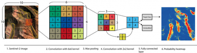
Artificial intelligence (AI) is the collective term for algorithms that are able to apply human-like reasoning to a specific problem and is one of the methods of data science. Machine learning is a subset of AI and describes the process of understanding, interpreting and processing data. The machine learning algorithm for feature detection uses a convolutional neural network (CNN). In a CNN, the algorithm makes a prediction based on two labels; in this situation, the MBES data points were labelled ‘seabed’ and ‘feature’. The CNN uses filters to recognize patterns in the datasets, and these filters consist of weights and biases that are adjusted during the training phase (Figure 1).

Dataset labelling

During training, a CNN is ‘taught’ to recognize seabed and features based on training datasets created by the AI developer. At the beginning of training, the neural network is not able to give definite results and requires this pre-processed data to determine the optimal filters. Training a neural network is an extensive process and requires a careful approach. During the training phase, the neural network is sensitive to underfitting and overfitting, which can only be observed after completion of the training session. An underfit model cannot model the training data or is unable to generalize to new data, whereas an overfit model models the training data too well, to the point that it adversely affects the model’s performance on new data. The training data must be prepared in such a way that as many different objects as possible are used. It is also important to label the coordinates as correctly as possible within the training datasets, as the filters are optimized based on the label definition from the training dataset. One sequence of going forward through the network with an estimation of where the seabed and features are and subsequently going backwards (called ‘back propagation’) to adjust the weights and biases is called an epoch. A training session consists of multiple epochs. After each epoch, training results are presented in the form of three parameters generated for both the training and validation part of the training session: ‘Loss’, ‘Accuracy’ and ‘Intersection over Union (IoU)’. Signs of underfit or overfit can be observed by producing a plot of the loss values.

The labels are binary, so a ‘0’ or a ‘1’. A human processor would probably assign ‘0’ to ‘seabed’ and ‘1’ to ‘feature’, as the feature is the item of interest. However, an inverse distribution was assigned during the research, as the seabed is present in a more consistent manner compared to a feature. Every feature on the seabed is unique in its own way, as different types of vessels sink in different ways and therefore end up on the seafloor in a variety of orientations and potentially different parts. If the algorithm was trained for wrecks, matching filters would have to be created for every situation and category of object. The hypothesis in this research is that this inverted training approach will benefit the creation of the filters and that the remaining data points (not defined as ‘seabed’) will form a cluster of points representing a feature. Even if the feature is not a wreck, it may still warrant an investigation and possibly a human classification after the AI detection. The differences between the normal and the used inverse distribution were not examined during this research.

CNN training

Processed MBES grid data for eight different wrecks in the North Sea was provided by the Royal Netherlands Navy and used in this research. Six wrecks were used to train the CNN while the remaining two were used to validate the CNN. Using the two validation datasets, the weights and biases were once more updated using back propagation, which is based on the differences between the prediction and the actual label assignation.

In the training phase, a total of six training sessions were initiated and equally divided into two groups, A and B. Each training session was a follow-up to the preliminary training session, to enhance the CNN parameters. The first three training sessions were considered failures due to the model focusing on undesired parts of the training dataset. After adjusting the training, the first two training sessions in group B showed promising results. The final training session showed signs of overfitting and was therefore also considered a failure. Therefore, only the fifth training session (the second from group B) was used for further testing against manual detection.

As mentioned earlier, training the machine learning algorithm is a difficult and time-consuming process, since insight into the training results can only be accessed after completion of the training session. In other words: the algorithm may be trained incorrectly, but this can only be understood in retrospect, thereby forcing the user to start the training session all over again with different training settings.

Not only is this repeated reinitiation of the training session a time-consuming process, but the computers’ hardware specification is also a bottleneck in the training process. Not having access to high-end hardware specs significantly increases the time required for a full training session. The arrival of AI has introduced a new approach to the utilization of a computer’s graphics processing unit (GPU). Originally, GPUs were designed to specifically handle rendering and other graphics applications, but in AI the GPU is used for small computations in large quantities. It is suited for this task due to its relatively higher number of cores compared to a central processing unit (CPU). Using a high-end GPU results in a significant decrease in training time.

MODI

The MODI proof of concept was built using the Python programming language and the open source Open3D-ML (machine learning) library. This MIT licensed library is specialized in handling 3D data and has the possibility of developing a machine learning tool. To circumvent GPU issues in the library at the time, MODI was created in Linux. Open3D-ML provides the user with several preset CNNs that can be used and adjusted to suit the application. MODI uses the Kernel Point CNN, which can manage 3D data to make predictions on it. MODI is however more than just the CNN kernel: it is a complete machine learning programme from which the machine learning kernel can be trained and the resulting 3D data can be visualized.

Detection reliability

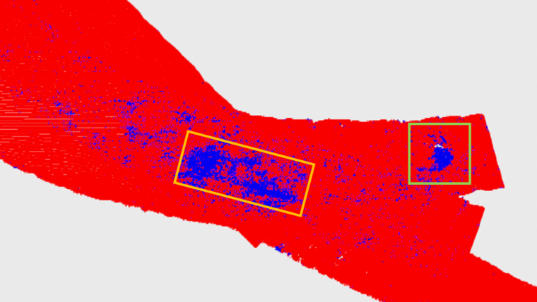
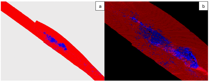
To produce unbiased statistical values, a dataset was required that was completely unfamiliar to MODI, meaning that the dataset must neither be used as a training or a validation dataset. Two wrecks, Boetak and Walsum 10, located to the south east of the island of Terschelling, were used as these foreign datasets (Figure 2, Figure 3). Both wrecks were surveyed in detail using an MBES by third year students on the Ocean Technology programme. A visual analysis showed that MODI was able to detect both wrecks, by representing the location of the wrecks with a large cluster of points correctly labelled as ‘feature’. Although Walsum 10 sank due to an explosion, causing the bow section to separate from the rest of the vessel, MODI was able to detect both of the sections by representing both sections as a large cluster of points correctly labelled as ‘feature’ (Figure 3).

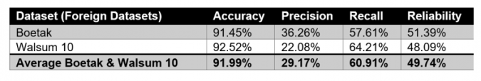
To produce statistical results on the predictions made by MODI compared to a manual selection, a confusion matrix was created. A confusion matrix consists of a 2*2 matrix with the true positive (TP), false positive (FP), true negative (TN) and false negative (FN) results. In this case, a true positive is a point correctly labelled as ‘seabed’ and a true negative is a point correctly labelled as ‘feature’. False positives and negatives are incorrectly labelled points. Using the confusion matrix, further statistical values were produced. The reliability for the two wrecks combined scored on average around 50%, as calculated from the weighted summation of the accuracy, precision and recall values. The accuracy is the ratio between the number of correct predictions (seabed and feature) and the total number of points. The precision is the ratio between the points correctly labelled as ‘feature’ and the total number of points correctly and incorrectly labelled as ‘feature’. The recall is the ratio between the points correctly labelled as ‘feature’ and the total number of points predicted as ‘feature’.

Conclusion

It is possible to create a machine learning tool to separate features from seabed in an MBES dataset. From the statistical analysis, it can be established that MODI’s reliability is currently at approximately 50%. However, from a visual analysis, a human can distinguish with the unaided eye that a feature is present, based on the large cluster of points marked as ‘feature’ at the location of the wreck and the relatively low amount of noise present. Based on these findings, an initial conclusion is drawn that a machine learning tool offers much potential to speed up the process of object detection. However, more research and training with different wrecks is required to increase the reliability of the tool.