Seabed Characterisation Using Wind Noise
The acoustic reflection coefficient of the seabed can be measured from the wind-generated noise of the ocean using a vertical line array of hydrophones suspended in mid-water. Results of experiments at several sites have previously been published and an example is presented here. The effect of the seabed on acoustic propagation from a source to receptor is illustrated by means of a simple formula.<P>
The formula predicts thatfor a highly reflective seabed the received acoustic power at moderate ranges could be at least four times that received from a single direct path, and higher still at long ranges. Such effects have been observed in previous work using a towed acoustic source.
Underwater ambient noise is continuously generated by wind and waves at the sea surface. As the noise propagates through a shallow water environment, it interacts with the seabed, which, along with other environmental factors such as the water sound speed variation with depth (sound speed profile), results in a variation in the noise intensity with elevation angle. This structure can be exploited to provide information about the acoustic properties of the seabed. Theoretical analysis shows that the difference between the received noise level for equal and opposite elevation angles about the horizontal is equal to the seabed reflection loss for that angle. The directional noise level can be measured by processing data collected on a vertical line array of hydrophones. The theory has been confirmed through experimental work [1,2,3].
Measurement Method
The difference in the received noise level for equal and opposite angles about the horizontal can be measured using a vertical line array of hydrophones suspended below the sea surface. Plane-wave beam-forming is used to calculate the array response, which resolves the directional structure of the noise field. Beams are formed for equal and opposite angles about the horizontal and the ratio of the noise intensity received in a downward-looking beam to that in the corresponding upward-looking beam is calculated for each beam pair. According to the theory, this gives the seabed reflection coefficient for the given beam angle. However, the limitations of the measurement system must be taken into account. The ability of the beam-former to resolve a plane wave depends on frequency, as the size of the vertical aperture in terms of the acoustic wavelength is a function of frequency. Furthermore, plane waves can only be resolved unambiguously at all angles up to the design frequency of the array (the hydrophones are spaced half a wavelength apart at the design frequency). Therefore, the measurement accuracy increases with frequency up to a maximum at the design frequency.
Systems Engineering & Assessment Ltd (SEA) has collected data using a vertical line array suspended below a freely drifting surface buoy. The array has 32 hydrophones and the design frequency is 4kHz, i.e. the hydrophone spacing is 18.75cm (with a nominal sound speed of 1,500m/s assumed).
Example of Measured Data
SEA has conducted trials at several locations around the UK coast with differing seabed types. The measured reflection coefficients have been compared with reference geoacoustic data in order to validate the method, with good agreement [3].
One such trial took place in August 2003 in the north-west approaches (NWAPPS) to the UK. The location was about 20 miles west of Barra Head. Reference geoacoustic data for the location show a seabed consisting of a thin layer of gravelly muddy sand overlying silty clay.
The array response was calculated using plane wave beam-forming in the frequency domain and time averaging over a 3-minute period, to give the spectrum noise level versus beam angle and frequency. Beam angles were chosen in order to obtain the reflection coefficient at regular angle intervals of 3°. The beam angles, whilst always symmetrical about 0°, can be at irregular intervals as Snell’s law is used to map angles at the seabed to angles at the array using the sound speed profile. The array response is shown in Figure 1.
The decrease in noise level towards the horizontal occurs due to the downwardly refracting water sound speed profile; there are some angles around the horizontal for which noise generated at the sea surface does not reach the array. This simply means that we cannot measure the reflection coefficient at these angles. At frequencies above ~1kHz, the vertical structure of the noise field is clear, from which we can use the down-to-up intensity ratio to derive the seabed reflection coefficient. The reflection coefficient is shown in Figure 2, plotted as reflection loss in dB per bounce, i.e. -10log10 R , where R is the intensity reflection coefficient given by the beam noise ratio.
The white area to the left of the plot corresponds to angles for which the reflection coefficient cannot be measured due to the water sound speed profile. The limitations of the measurement system discussed earlier are visible in Figure 2, and the useable frequency band extends from about 1kHz to just below 4kHz.
Figure 2 shows a highly reflective seabed, with a critical angle (where loss changes from low to high) of around 40SDgr. The reflection loss near normal incidence is quite low, being only around 6dB. These characteristics are as expected for a seabed with a hard upper layer, and the measured reflection coefficient is in good agreement with a modelled reflection coefficient constructed from reference geoacoustic data [3].
Data sets were also collected at a location east of the port of Blyth on the north-east coast of England, and at a location approximately halfway between the island of Raasay in Scotland and the Scottish mainland. For the Blyth location, reference geoacoustic data show a layer of silts and muddy sand overlying a layer of very soft mud. A detailed geoacoustic model for the Raasay location was not available, but the seabed is known to consist of very soft mud. Details and measured reflection coefficients for both locations have been presented in the Hydrographic Journal [3].
Averaged Reflection Coefficients
The reflection coefficient can be derived over the useable frequency band of the array. In all three cases, the results are essentially frequency-independent over this band. We can therefore average the reflection coefficients over the band between 1.5 and 3.5kHz to produce a single angle-dependent intensity reflection coefficient for each case. The results are shown in Figure 3, in which the variation of reflection coefficient with seabed type is clear. Note that averaging over frequency is a valid approach only when there is little variation in the reflection coefficient with frequency, as in these cases. If there were strong layering effects for example, an averaged reflection coefficient could differ from that at a particular frequency.
As discussed earlier, beam angles were chosen in order to obtain the reflection coefficient at regular angle intervals of 3°. For the NWAPPS trial (see Figure 2) and Blyth trial (see [3]), no values are available below 9° due to the sound speed profiles. For the relative intensity calculation described below, reflection coefficient values on a continuous grid from 0° to 90° are required, hence the values must be extrapolated down to 0°. As the value at 0° is unity by definition, interpolation is carried out between unity at 0SDgrand the first measured value at the corresponding angle.
Figure 4 shows the reflection coefficients after extrapolation and interpolation, plotted as intensity reflection coefficient R rather than reflection loss, where reflection loss is given by –10log10 R . The angle spacing is still 3°, but now extends down to zero. The circles indicate measured values.
Effect on Acoustic Propagation
Here we illustrate the importance of the seabed in acoustic propagation by examining the relative increase in noise intensity from extra acoustic path contributions due to a reflective seabed over that due to the direct acoustic path only. The case considered is for a source at the sea surface (e.g. a ship) and receptor on the seabed. Both source and receptor are assumed to be omni-directional. The geometry is illustrated in Figure 5. The environment is assumed to be isovelocity, i.e. spherical geometrical spreading applies along each path. Figure 5 shows the direct and single bottom bounce paths. Clearly, there will be multiple bottom bounce paths, each of which has an equivalent number of surface bounces.
We have already derived frequency-independent seabed reflection coefficients by averaging over the useable array processing band. Water volume loss and surface bounce loss are ignored in the formulation below, in order to obtain a frequency-independent result. The result is therefore most applicable to low frequencies (those where shipping noise dominates) and calm sea surfaces.
The path with n bottom bounces suffers intensity reduction given by the reflection coefficient at the bottom angle for the path raised to the power n , as well as geometrical spreading. The quantity of interest is the ratio of the intensity from all contributing paths to that from the direct path only.
Firstly, although in theory there is an infinite number of contributing paths, we start by including only the path with a single bottom bounce. As would be expected, the intensity ratio asymptotically approaches a value of 2, i.e. the direct and bottom bounce paths are received with about the same intensity. This occurs because at long ranges the path lengths are similar and at the correspondingly low bottom angles the reflection coefficient approaches unity. Clearly, the ratio of 2 will be approached fastest for the seabed whose reflection coefficient approaches unity fastest.
We now increase the number of paths until there is no difference in the result, i.e. approximate the sum to infinity. Including 30 paths is sufficient.
For the most highly reflective case, i.e. the NWAPPS seabed, the intensity ratio reaches a value of 4 at about 3km. This is significant: the acoustic power received is four times that from the direct path only. This occurs at about 4km for the Blyth seabed, and the ratio remains below 4 out to 10km for the Raasay seabed.
Although no data are available to SEA for a source on the sea surface and receiver on the seabed, the effect of additional contributions from the seabed has been observed with measured data, using a single frequency tone transmitted from a towed source and received on the vertical line array [4]. The observed increase in acoustic intensity over that expected from a single direct path agrees well with the above formulation, including the difference between high and low reflectivity seabed types.
Conclusions
A method for seabed acoustic characterisation using only the wind-generated noise of the ocean has been discussed, and experimental results shown. The effect of different seabed types on acoustic propagation has been examined using a simple formula. The formula predicts that for a highly reflective seabed, the received acoustic power at moderate ranges could be at least four times that received from a single direct path, and higher still at long ranges. Such effects have been observed in previous work using a towed acoustic source.
Acknowledgements
The work on seabed reflection coefficient measurement was funded by the UK MoD Research Acquisition Organisation. The copyright in this work vests in Systems Engineering & Assessment Ltd. The author acknowledges Dr Chris Harrison of the NATO Undersea Research Centre for his extensive research in this field andfor helpful advice in the early stages of the work.
References
1Aredov, A.A., and A.V. Furduev, 1994: Angular and Frequency Dependencies of the Bottom Reflection Coefficient from the Anisotropic Characteristics of a Noise Field. Acoustical Physics , 40(2), pp. 176-180.
2Harrison C.H., and D.G. Simons, 2002: Geoacoustic Inversion of Ambient Noise: A Simple Method. Journal of the Acoustic Society of America , 112(4), pp. 1377-1389.
3Donnelly, M.K., 2006: Acoustic Characterisation of the Seabed Using Wind Noise. The Hydrographic Journal , 122, October.

Value staying current with hydrography?
Stay on the map with our expertly curated newsletters.
We provide educational insights, industry updates, and inspiring stories from the world of hydrography to help you learn, grow, and navigate your field with confidence. Don't miss out - subscribe today and ensure you're always informed, educated, and inspired by the latest in hydrographic technology and research.
Choose your newsletter(s)