Improving Overall Resolution of Bathymetric Survey
Integrated Use of Multi-beam Echo Sounder and Towed Interferometric Sonar
Designing offshore engineering facilities requires large amounts of information. To acquire it, suites of engineering and geophysical surveys are run, which as a rule include such techniques of seabed and sub-bottom investigation as seismic profiling, acoustic, magnetic and bathymetric surveys. Obtaining accurate and detailed seabed bathymetry is extremely important because the quality of other surveys depends on the quality of the bathymetry.
One of the most accurate and cost-effective ways to acquire high-resolution bathymetric data is the use of shipborne bathymetric systems such as multi-beam echo sounders (MBES) or interferometers. The drawback of this method is that the resolution of seabed imaging decreases with water depth. Use of bathymetric systems installed on remote operated vehicles (ROV) or autonomous underwater vehicles (AUV) allows for the acquisition of high-accuracy high-resolution data, though survey costs considerably increase due to longer acquisition time and higher cost of equipment. Presently, towed acoustic complexes are widely used, with a combination of a sub-bottom profiler (SBP) and an interferometric sonar (IFMS) mounted on a single tow fish. Their use makes it possible to acquire high-resolution data, though data accuracy degrades with the increase of tow line length. A trade-off may be achieved through combined use of a shipborne MBES and a towed acoustic complex with a towed IFMS (TIFMS), which makes it possible to integrate the accuracy of MBES data and the resolution of IFMS data without considerable cost increase (Figure 1). That implies the availability of a technique for integrated processing of MBES- and IFMS-acquired bathymetric data.
In 2007-2009, engineering surveys were conducted for designing subsea infrastructure facilities to develop the Shtokman gas-condensate field. Bathymetric surveys were acquired by shipborne MBES Reson SeaBat 8111. The Teledyne Benthos C3D acoustic system was also used, in which a seismic profiler and a TIFMS are combined, with an associated Marine Magnetics SeaSPY magnetometer. A technique was developed for integrated processing of bathymetric data from different sources, with different accuracy and resolution, for improvement of overall survey accuracy.
Survey Conditions
The shipborne MBES was mounted on the side pole of R/V Akademik Golitsyn. The tow fish was towed 20-25 m above the seabed at a speed of 3.5-4kt. Sea depth in the survey area was 50-370m. The length of the tow line varied from 50 to 1050m (tow depth multiplied by 3-3.5). For tow fish positioning, the Kongsberg HiPAP 500 USBL system was used. The tow fish was also equipped with an iXSEA Octans fibre optic gyro/motion sensor.
Due to the poor quality of the phase measurements, TIFMS measurements in the near and far fields (closer than 30m and farther than 140m from nadir) had to be rejected .
Data Accuracy and Resolution
The resolution of an MBES survey depends on the dimensions of zones ensonified by beams, which increase with sea depth, beam width, and tilt angle of a beam (for MBESs with fixed beam width). Vessel yaw, pitch and roll cause shrinkage and dilatation of ensonified zones, which affects the resolution. In addition, the position of a reflection point at the seabed does, in general, not coincide with the position of its image . Thus, seabed imagery suffers from distortions that are manifested in the apparent flattening of the terrain.
The resolution of a TIFMS survey depends on sampling rate and working range. When towed at a small altitude, the resolution of seabed imagery is high and relative distortions of relief features are insignificant . However, the accuracy of its absolute position is lower than that of the MBES, because the tow fish is at a significant distance from the vessel and its position is determined by the USBL. That is why the TIFMS image is also distorted, though its distortion manifests itself as a shift of the image relative to the true seabed.
Survey accuracy and resolution for the said conditions are shown in Table 1. It illustrates that MBES has a better accuracy, while TIFMS has a better resolution.
Essence of Technique
Usually, processing of bathymetric survey data results in creating a digital terrain model (DTM). DTMs are used for solving various engineering problems and they have the same advantages and disadvantages as the data from which they are generated. That is, the advantage of the TIFMS DTM is its resolution, while that of the MBES DTM is accuracy. Due to its higher accuracy, an MBES DTM can be considered to be closer to the true seabed by position. A TIFMS DTM, in turn, is closer to the true seabed by detail level.
An obvious way to obtain a DTM merging both advantages is to draw a TIFMS DTM nearer to an MBSS DTM and, subsequently, nearer to the true seabed relief. To solve this problem, it is necessary to find a method for determining optimal shifts for cells of a TIFMS DTM and introducing them.
Mathematically, an assemblage of DTM depths can be presented as a random function of coordinates. If two DTMs with equal cell sizes constructed from data of equal accuracy and resolution describe one and the same seabed area, corresponding values of these functions should coincide within the accuracy of measurement. However, due to the fact that in our case these parameters differ, values of the functions (depths) differ from each other.
Let us assume that a TIFMS DTM is not shifted relative to an MBES DTM and hence depth value difference is caused by resolution difference only. A change in depth of the MBES DTM is accompanied with a change in depth of the TIFMS DTM in the same direction. Depth differences will, in general, vary, though their assemblage will tend to an average depth difference. Hence, a positive linear correlation exists between the two DTM functions. As a quantitative measure of similarity, the Pearson correlation coefficient (PCC) can be used. The better the coincidence between the DTMs, the higher the PCC value. With entire coincidence of the two DTMs, the PCC will equal 1.
It is quite obvious that in a case of shifted TIFMS DTM, correlation will be weaker than in a case without shifting. Consequently, a maximum PCC can serve as an indicator of closest fit of the DTMs. The problem of drawing a TIFMS DTM nearer to an MBES DTM can be solved by analysing this indicator. The problem is split into two stages – the horizontal and vertical approximations.
Horizontal Approximation
As was said above, a difference in accuracy of determining depth positions manifests itself as a shift of TIFMS DTM regions relative to the MBES DTM that is assumed the true seabed relief. Shifts are of smooth character and can be assumed constant within certain limits.
To solve the problem, both DTMs are tiled into matrices. The size of the TIFMS matrices follows from the size of evenly shifted parts of the swaths. The size of the MBES matrix is greater than that of the IFMS matrix by the maximum expected shift value (Figure 2). For correct estimations, the TIFMS matrix is thinned and smoothed to the size of the MBES DTM cells.
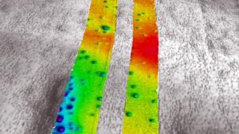
By shifting the TIFMS matrix step-by-step within the MBES matrix, a PCC is calculated for each position. These values are then arranged into a PCC array (Figure 3). The position with the maximum PCC value corresponds to the sought horizontal shift of the IFMS matrix. Linearly interpolated shift values are then applied to the coordinates of each point of the original non-thinned IFMS DTM (Figure 4).
A more generic way is to introduce shift values in coordinates of IFMS track line points. In this case, the positioning of SSS and SBP data can also be corrected, because all devices are combined in the same tow fish.
Vertical Approximation
The vertical mismatch of TIFMS and MBES DTMs is caused by differences in depth determination accuracy and it also can be corrected. For this purpose, both DTMs are tiled into identical matrices with a size defined by estimated dimensions of evenly vertically shifted parts of swaths. Differences of average depths are calculated for each pair of matrices. These differences are then introduced into depths of each point of the TIFMS DTM.
Approximation Accuracy
The accuracy of the described technique of fitting TIFMS data to MBES data can be analysed based on the distribution of PCC values in PCC arrays for various seabed types (Figure 5).
1. On a flat and featureless seabed (Figure 5a), PCC values in the array vary insignificantly, and do not show a well-defined maximum. In some cases, false maximums are defined. This is the case of the lowest matching accuracy.
2. A seabed dissected by prolate features with a distinct general trend such as troughs or crests (Figure 5b) is characterised by higher PCC values in the direction along the features. The matching accuracy is higher in the direction across the features and lower in the direction along the features.
3. Dissected relief (Figure 5c) is most readily discernible and, hence, a PCC distribution shows a well-defined maximum.
Other Methods
Similarity of DTMs can also be analysed using the least-squares technique. In this case, the sum of depth differences squared is calculated at each point for each pair of matrices. The position where this sum is minimal is the indicator of the best match of the DTMs. A disadvantage of this technique is its dependence on vertical distance between DTMs. This makes it impossible to estimate the degree of similarity.
Conclusion
Use of the described method of integrated processing of bathymetric data allows approximating high-resolution data to high-accuracy data. In addition, the accuracy of SSS and SBP data can be improved based on this method. The best approximation results are achieved in dissected seabed areas. The method helps to improve the overall bathymetric data performance without expensive techniques of field acquisition.
Acknowledgments
Kleschin S.M. (PeterGaz LLC, Russia)
| Sea depth, m | MBES | TIFMS | ||||
| Average accuracy of reduced depths, m | Average positioning accuracy of reduced depths, m | Average depths density, depths/m2 | Average accuracy of reduced depths, m | Average positioning accuracy of reduced depths, m | Average depths density, depths/m2 | |
| 50 | 1.2 | 5.0 | 0.44 | 3.5 | 4.7 | 15 |
| 90 | 1.3 | 3.9 | 0.28 | 3.5 | 4.9 | 15 |
| 130 | 1.4 | 3.8 | 0.21 | 3.5 | 5.4 | 15 |
| 170 | 1.4 | 4.0 | 0.17 | 3.5 | 5.9 | 15 |
| 210 | 1.4 | 4.3 | 0.15 | 3.5 | 6.5 | 15 |
| 250 | 1.4 | 4.6 | 0.13 | 3.5 | 7.2 | 15 |
| 290 | 1.5 | 5.1 | 0.12 | 3.5 | 7.9 | 15 |
| 330 | 1.5 | 5.6 | 0.10 | 3.5 | 8.6 | 15 |
| 370 | 1.5 | 6.0 | 0.10 | 3.5 | 9.4 | 15 |
Table 1: Accuracy and resolution of MBES and TFMS surveys.

Value staying current with hydrography?
Stay on the map with our expertly curated newsletters.
We provide educational insights, industry updates, and inspiring stories from the world of hydrography to help you learn, grow, and navigate your field with confidence. Don't miss out - subscribe today and ensure you're always informed, educated, and inspired by the latest in hydrographic technology and research.
Choose your newsletter(s)