Integrating Offshore Tide Model Output with Onshore Observations

The National Oceanic and Atmospheric Administration (NOAA) develops tide correctors for reducing hydrographic survey soundings to Chart Datum by using the Tidal Constituent and Residual Interpolation (TCARI) software to interpolate harmonic constituents (HCs), tidal datum elevation relationships and water level residuals from observations. Due to the complex tidal regime and limited coastal observations in the Bering Sea, the error associated with tide correctors generated from the TCARI interpolation exceed the 45cm National Ocean Service standard in some offshore areas. In an effort to develop a higher quality tide corrector, a method of blending offshore HCs from high-resolution tide models and the onshore observations was explored.

(Due to the nature of the images and the table, please see them in the digital magazine edition of September 2015)

This paper presents the general concept and operational feasibility of this approach. A regional tide model was used to provide the offshore HCs in the Bering Sea. The main objective of this study was to evaluate if the integration of offshore, modelled harmonic constituents with onshore observations improves the accuracy of tide correctors in the Bering Sea.

The Limitation of Current Zoning Scheme in the Bering Sea

TCARI is a method of interpolation to derive water level correctors that reduce hydrographic soundings to Chart Datum (MLLW). The accuracy of TCARI largely relies on the spatial distribution and availability of data. Currently, there are only four permanent NOAA operating water level stations along the Bering Sea coastline up to the Bering Strait and 20 additional stations with published HCs. Given the 2,000km shoreline along the Bering Sea coast, the geographic distribution of observed data is very sparse, resulting in high TCARI errors.
In addition, the interpolation accuracy is impacted by the tidal complexity as interpolation across complex tidal regimes increases the uncertainties of the solution. The tides in the Bering Sea are complex for several reasons; the first is the existence of several diurnal and semidiurnal amphidromes. An amphidromic point is a point of zero vertical displacement of one harmonic constituent of the tide. The amplitude of that harmonic constituent increases with distance away from this point and the phase of the constituent changes continuously around the central point (Figure 1). The direct interpolation of observations from coastal stations results in offshore solutions that have errors greater than the 45cm specification.

Tide Model Evaluation 

A regional tide model developed by Foreman et al. (2006), which assimilated satellite altimetry data, was used to provide additional HCs. Before being incorporated into a TCARI solution, the modelled HCs were evaluated by comparing them with the published HCs at NOAA stations. For this evaluation the principle semidiurnal constituent, M2, and principle diurnal constituent, K1, were used for comparison.

An error was computed for each constituent at each location which combines the amplitude and phase differences. The relative error (%) was calculated by dividing the error by the observed amplitude of the constituent, which provides a measure of the relative performance of the model for each constituent. However, it should be noted that for constituents with minimal amplitude, any discrepancy will result in a large relative error. The error values for M2 ranged from 6mm to 35cm and K1 ranged from 6mm to 16cm. The relative error values for the M2 constituent ranged from 2.4% - 180% of the observed amplitude, and from 3.8% - 90% for the K1 constituent. Given these discrepancies, tide reductions derived from the tide model alone would not meet NOAA’s hydrographic survey specifications.

Tide Model Integration

The output from selected offshore model output points were combined with the observations from onshore stations for TCARI interpolation so that the model results contributed more to the interpolated HCs in the offshore regions and the onshore observations contributed more to the interpolated HCs in the nearshore regions. Two ways of selecting model points were investigated. One method used a programme that automatically selects evenly distributed model points throughout the TCARI domain. The other involved a manual selection of model points based on spatial distribution of modelled amphidromes.

Four different scenarios of integrating model points were evaluated in this study. They are described by a parameter G for the grid spacing, and a parameter D for the minimum distance between model points and tide stations. Three evenly distributed scenarios are: 100km grid spacing and 30km tide station distance (G100 D30); 80km grid spacing and 50km tide station distance (G80 D50); 50km grid spacing and 25km tide station distance (G50 D25). The fourth scenario is 129 model points clustering around the locations where there are suspected amphidromes (Figure 2). Combining these four blended scenarios, the solution using only data from operating tide stations, and the tide model output itself, a total of six scenarios were used for comparison with data collected offshore in the 1980s.

Comparison of Errors among 6 Scenarios

As part of two Pacific Marine Environmental Lab (PMEL) studies in the Bering Sea, pressure gauges were deployed from the tip of the Seward Peninsula south to the end of the Alaskan Peninsula (Pearson et al., 1981 and Mofjeld, 1986). The HCs derived from the data of 24 of these gauges were used as ground-truth information for comparison between six scenarios.

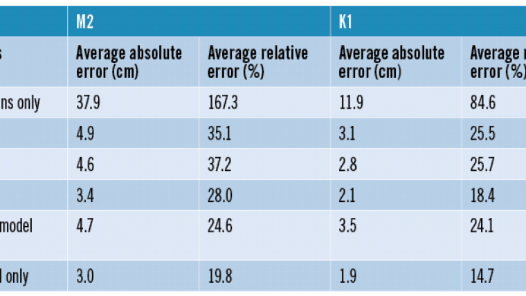
The results for the M2 and K1 constituent comparisons are shown in Table 1. Table 1 indicates that the addition of model output into a TCARI solution significantly reduced the error for M2 from 37.9cm to 3.4cm and K1 constituents from 11.9cm to 2.1cm, in the best cases. Accordingly, the relative error for M2 was reduced from 167.3% to 24.6% of the observed amplitude and from 84.6% to 18.4% for K1.

M2 and K1 Contours in the Bering Sea

Phase contours of the M2 and K1 constituents from the six scenarios were exported from TCARI to allow for the comparison of the different solutions in the Bering Sea (Figure 3 and 4). The tide-stations-only plot did not reveal any single M2 amphidromic point, while the other five solutions, including the tide-model-only solution, show several amphidromic systems. The M2 contours (Figure 3) from the clustered-model-points scenario were most consistent with those from the tide model. The G50 D25 evenly-distributed scenario was similar to the clustered solution, but the significant increase in the number of points would present an operational limitation. The G100 D30 and G80 D50 evenly-distributed solutions did not resolve all of the suspected M2 amphidromes that the Foreman tide model shows.

Plots of the K1 phases in Figure 4 suggest that the clustered solution most similarly reproduced the two suspected diurnal amphidromic points. The tide-stations-only solution resolved a full amphidromic point off of the south-western tip of the Seward Peninsula, which is consistent with Pearson (1981) (see Figure 1), while the model only identified it as a partial amphidromic point. The tide-stations-only solution did not show the amphidromic point in western Bristol Bay that was captured by the Foreman tide model, as well as all four blended solutions.

Discussion and Future Work

An additional sensitivity test was performed using the evenly distributed model points (Figure 5). The goal was to test the sensitivity of the gridding distance parameter G by setting it to 6 different values: 400km, 300 km, 200km, 100km, 50km, and 20km. Additionally, the tide station distance parameter D was fixed at 50km. The average error reduced significantly when model output spaced at 400km was included in the TCARI solution. This improvement was less dramatic when reducing the density parameter further. The trend was the same for both the M2 and K1 constituents. These types of sensitivity tests are important to maximise results while minimising computer processing time. For the Bering Sea, the use of model output at the 400km grid level (8 model points) provided an error within the specifications for NOAA hydrographic surveys, despite not resolving all of the complex tidal features.

This method will continue to be evaluated in regions of well-understood tidal physics such as Chesapeake Bay and then implemented for tide reduction operations in the near future.

Acknowledgements

The authors of this publication would like to thank the leadership of NOAA’s Center for Operational Oceanographic Products and Services (CO-OPS) and Office of Coast Survey (OCS), as well as all the employees who contributed to this project including Louis Licate from CO-OPS, and Lei Shi and Barry Gallagher from OCS.

More information

Foreman, M.G.G.; Cummins, P.F.; Cherniawsky, J.Y. and Stabeno, P., 2006. Tidal energy in the Bering Sea. Journal of Marine Research 64, 797-818.

Huang, L., Wolcott, D., Licate, L., Wong, J., Gallagher, B., Meyer, E. and Shi, L., 2014. Integrating Offshore Hydrodynamic Model Output with Onshore Observations to Improve Correctors to Hydrographic Survey Soundings, Proceedings of U.S. Hydro 2014 Conference, The Hydrographic Society of America, Newfoundland and Labrador, Canada, 16pp.

Mofjeld, H.O., 1986. Observed Tides on the Northeastern Bering Sea Shelf. Journal of Geophysical Research 91, 2593-2606.

Pearson, C.A., Mofjeld, H. O. and Tripp, R. B., 1981. Tides of the Eastern Bering Sea Shelf. In The Eastern Bering Sea Shelf: Oceanography and Resources, Hood, D and Calder, J. A. Calder (eds), Vol. 1, USDCS/NOAA/OMPA, pp. 111-130.

Shi L., Wang J., Myers E. and Huang, L., 2014. Development and Use of Tide Models in Alaska Supporting VDatum and Hydrographic Surveying. Journal of Marine Science and Engineering, 2(1), 171-193.