Satellite Positioning
Within the last twenty years Global Positioning System (GPS) receivers have revolutionised navigation. Integrated devices are capable of providing time, position, height, direction, heave and attitude to accuracies of a few nanoseconds time, 1cm position or 0.01 degree heading. All potentially displayed on a digital chart background with radar and auto-identification system overlays. In this first of two articles we look at current Satellite Positioning systems, how they work and how we can make them better. In a second article, to appear next month, we explore the future development of Satellite Positioning and the implications for navigation.
How does Satellite Positioning work? Switch on a satellite-positioning receiver and it gives a position within a minute or two, but what happened during that time? Why are some receivers more accurate (and more expensive) than others, and why do I need Differential GPS (DGPS), Wide Area Augmentation System (WAAS), Global Satellite Based Augmentation System (GSBAS), Real Time Kinematic (RTK) and other technical acronyms?
Satellite Navigation
Each Global Navigation Satellite System (GNSS) satellite transmits a number of carrier frequencies upon which are a number of codes. These include timing intervals, satellite positioning information, an ionospheric model and a code specific to the satellite, allowing multiple satellites to transmit on the same frequencies. Receivers may use some or all of these frequencies and codes and this will determine to a large extent the positioning performance. Figure 1 illustrates the basic principles of satellite positioning.
The GNSS receiver has multiple receiver channels and generates its own internal version of the GNSS signal to compare against the signals received. The difference in time between these two can be converted to a pseudorange distance by using the speed of light. An ephemeris (set of satellite position information) stored in the receiver may then be used to determine initial receiver position by trilateration. We need three simultaneous pseudoranges from different satellites geometrically well spaced to solve for latitude, longitude and height. The satellites have onboard atomic clocks synchronised via the system Master Control Station to a master atomic clock on the ground that contributes to the fundamental timing infrastructure of the planet. Synchronised atomic time standards are too expensive to put in typical satellite-receiver user equipment, so a fourth satellite pseudorange observable is required to calculate the receiver clock offset to the synchronised system atomic time.
Once you have an initial position and receiver clock offset the receiver can tighten the tracking loops and start decoding the new ephemeris information plus ionospheric model, and this in turn will improve the position performance. Additional pseudoranges can be used to provide a confidence check of the position calculation or to estimate other variables to improve position accuracy. The GNSS-determined height is referenced to a mathematical approximation of the earth’s surface, typically the WGS84 or GRS80 spheroid. However, what most users are interested in is the Mean Sea Level: one particular equipotential surface. Variations in crustal density and thickness cause undulations in the mean seal level that may be represented by means of a geoid model with respect to the spheroid. Geoid models such as EGM96 are often built into GNSS receivers such that the height output can be either spheroid or orthometric (mean sea level).
Code measurements have a relatively coarse resolution. A common method used to improve upon this is to use the carrier-phase signal count to smooth these over time. Carrier-phase measurements can also be used interferometrically to determine highly accurate relative orientation between multiple GNSS receivers on the same ship/platform. This is the technique employed by GNSS-based heading sensors and precise roll determination systems for multi-beam bathymetry sensors. The distance between GNSS antennae and the quality of GNSS receiver determine heading-and-roll accuracy.
Signal Variability
To get more accurate positioning we need to consider more variables, as shown in Figure 2. Orbit is the difference between the broadcast position and the true position. On 14th August 2006, for GPS this was as much as 10.7m (PRN30), with an average of 1.90m for all satellites throughout the day. Clock for each satellite varies with respect to the master control clock. On 14th August 2006 GPS clocks varied by as much as -4.0m (13ns) to +5.0m (17ns), with PRN01 having the greatest total variation during the day: 6.5m (22ns). The combination of GPS orbit and clock offsets are represented as the User Range Error (URE). URE as reported by the GPS Operations Centre at Space Command Schriever Air Force Base has recently been in the range 0.5-2m. For Glonass, URE for May 2006 was reportedly in the range 5-11m.
Ionosphere consists of a number of layers between 50 and 1500kms altitude, with negatively charged electrons plus positively charged atoms and molecules. The total electron content (TEC) is based upon solar activity which is related to time of day, position with respect to the geo-magnetic equator and where we are in the eleven-year solar cycle. We are currently approaching a solar-cycle minimum but TEC can still be high, especially at 15 degrees north and south of the geo-magnetic equator at 14:00 local time. TEC affects each frequency differently and slows down pseudoranges but advances carrier phases by equal amounts. A ratio of dual-frequency GNSS measurements can be used to correct for TEC-in-duced effects. Alternatively, a position and time-based ionospheric model can be used for single-frequency receivers. This typically corrects for 40-60% of TEC. Ionosphere models use an altitude of 350-400kms and provide a regular grid of zenith TEC values which have to be converted to slant delays via an elevation look-angle mapping function.
Troposphere extends up to an altitude of 40kms, although the majority of variability is concentrated within the first 8kms above the poles and up to 16kms in equatorial areas. The tropospheric delay is frequency-independent for GNSS signals and consists of two components. The hydrostatic component represents approximately 2.4m zenith delay at sea level, whilst the wet component is up to 0.4m zenith delay. The troposphere can be modelled over a large area by weather sta-tions and multiple GNSS base-stations; however, the wet component remains difficult to compute accurately and with sufficient granularity. For non-zenith satellites, the hydrostatic and wet-zenith delay components have to be mapped to slant delays via elevation look-angle functions, and this can increase the total delay to as much as 28m at 5degrees elevation. Alterna-
tively, a fifth variable can be introduced into the satellite positioning algorithm to model local tropospheric zenith delay; this requires the availability of five satellite ranges.
Multipath results in multiple signals at the receiver, the strongest direct signal arriving first and reflected and refract-ed signals arriving later due to the longer path travelled. GNSS-receiver antennae can use a large groundplane to minimise multipath signals reflected from beneath the antenna. However, this has a drawback in a marine environment when the mast is tilted, because the groundplane will exclude some good direct low-elevation satellite signals. Modern GNSS receivers use signal-processing techniques to further reduce multipath signals.
When a receiver is locked to a signal it knows when the code edge is due and can take a signal sample before and after (called the sampling window) to detect the code edge before the multipath delayed signal arrives. The size of the sampling window will depend upon the sophistication of the receiver and this will determine the volume of multipath that can be rejected by this method. This technique works best for multipath that has delay longer than the sampling window. Short delay multipath will still be in the sampling window, so for best performance the antenna should be positioned away from nearby flat structures or should use some form of groundplane. More advanced multipath techniques exist, such as Double Delta, but these are beyond the scope of this article. Figure 3 shows a typical workboat scenario with both multipath and satellite visibility issues.
Receiver hardware, antenna and software have channel biases and delays that can be calibrated and compen-sated for with the satellite-positioning algorithm. Earth tides are due to solar-system gravitational effects that cause the Earth's crust to move by as much as 55cm vertically at the equator, plus a slight horizontal component. This Moon and Sun dominated effect can be accurately modelled.
Augmentation
Augmentation systems provide additional information for these secondary variables. They transmit this in real time via radio or communication satellite so that the receiver can apply this information to improve positional accuracy.
How these secondary variables are determined will affect improvement in position. The ship far offshore, on the other hand, has a very different signal path (R2), with ionospheric and tropospheric differences relative to the base. So the two ships are considered spatially decorrelated. The RB measured by the base receiver can be compared to the distance between the broadcast satellite position and the known coordinates of the base-station to produce a pseudorange difference. This is the accumulation of all the corrections for that particular satellite to the base at that time. The position of the offshore ship will be less accurate than the inshore ship when using the augmentation signal transmitted from the single base, because accuracy is directly proportional to the distance from such. The worldwide Beacon DGPS system uses the above principle, transmitting corrections on marine radio-beacon frequencies.
Some augmentation systems, such as Network Real Time Kinematic and Wide Area Phase, determine models for second-ary variables from a regional network of bases and so reduce the spatial decorrelation effect for the network area. The corrections from these networks are distance dependent outside their coverage area, which limits their benefit offshore.
Satellite Based Augmentation Systems, such as the Wide Area Augmentation System (WAAS) and European Geostationary Navigation Overlay Service (EGNOS), use a regional network to determine orbital and clock corrections, plus an ionospheric model. These have been designed for aeronautical navigation, the signals being freely transmitted from geo-stationary satellites using the same L1 frequency as GPS. Thus making them readily usable for offshore positioning, achieving accuracies of a few metres within their applicable areas.
Another technique, GSBAS, uses a large GNSS global tracking network to determine very accurate and precise orbit and clock variables that are transmitted to ships and other users via dedicated communication satellite links. The ionosphere is directly measured using a dual-frequency receiver at the ship, and the navigation algorithm models both troposphere and multipath from redundant satellite observables over time.
Earth tides are well known and compensated for by a time-and-position-based model. Receiver and antenna biases are hardware-calibrated and used in the navigation algorithm. This method is capable of producing decimetre accuracy irrespective of the distance from the network base-stations; the offshore ship has just as accurate a position as the inshore ship.
Currently, 29 GPS satellites provide two frequencies, L1 and L2, with the civilian Coarse Acquisition Code (C/A) on L1 and the Military P Code encrypted to Y Code available on both L1 and L2. The first of eight GPS IIR-M satellites with the new L2CM, L2CL, L1M and L2M codes was launched on 25th Sep 2005. A May 2006 presentation showed that fourteen GPS satellites were a component of Nav failure. As of 1st August 2006 there were twelve operational Glonass satellites, plus two satellites switched off and two expected to be declared operational within the next sixty days. Transmissions are 'frequency division multiple access' (FDMA), requiring the receiver technology to support a much wider frequency front end, which affects receiver end-user costs and performance.
WAAS is now fully operational, covering USA, Alaska, Hawaii and Puerto Rico. The performance level stated by the Federal Aviation Authority for L1 receivers equipped with WAAS will be 7m horizontal and vertical. Consumer handheld GPS manufacturers have been advertising a performance of less than 3m. WAAS performance for a static dual-frequency receiver on the West Coast of the USA in July 2006 shows an accuracy over 24hours of 0.3m horizontal and 0.4m vertical (1 sigma).
EGNOS signals which will eventually provide a SBAS correction stream for Europe are not yet authorised for use. Testing with a static dual-frequency GPS receiver in Germany in July 2006 showed an accuracy of 0.5m horizontal and 0.7m vertical (1 sigma).
In addition to GPS and Glonass, there is China's Beidou (Big Dipper) triple-satellite constellation. Launched on 31st October 2000, 21st December 2000 and 25th May 2003 at longitudes 80, 140 and 110.5 degrees East respectively, it was declared operational in 2004. The system uses bi-directional ranging to provide communication and 100m horizontal positioning to authorised users in South East Asia. There are three main tracking stations for orbit determination: at Jamushi, Kashi and Zhanjiang. The satellites transmit at 2491.75 +/-4.08MHz and the ground receiver can transmit back to the satellites on 1615.68MHz.
Concluding Remarks
In this very brief synopsis of satellite positioning we have reviewed the current operational GNSS, how they work, their operational limitations and how different augmentation methods can improve their accuracy and usability.

Value staying current with hydrography?
Stay on the map with our expertly curated newsletters.
We provide educational insights, industry updates, and inspiring stories from the world of hydrography to help you learn, grow, and navigate your field with confidence. Don't miss out - subscribe today and ensure you're always informed, educated, and inspired by the latest in hydrographic technology and research.
Choose your newsletter(s)