When is it Advantageous to Maximise Swath Width?

Production seafloor surveys for hydrography require careful planning, balancing many factors for operational efficiency. Requirements for meeting International Hydrographic Organization (IHO) standards for horizontal and vertical uncertainty and object detection must be met, while maximising the coverage area in as short a time as possible. One may then pose the question, “When is it advantageous to maximise the swath width?” The answer might be surprising.

Background IHO requirements

To meet IHO requirements for vertical uncertainty, swath mapping has traditionally operated with swath widths covering an angular sector from nadir of +/- 65 degrees or less. Uncertainty in the measurement of the ship’s roll, combined with that of refraction, when propagated to uncertainty in the final depth at the edge of the swath can prove limiting, particularly when the sounder’s depth measurement itself is a significant portion of the uncertainty budget.

However, modern echo sounders now routinely produce soundings whose uncertainty can be as low as 0.1% of the water depth or lower. When conditions are favourable, the lower sounding uncertainty, combined with high-quality motion sensors, whose attitude uncertainty is also low, allows an increase of the swath width while still meeting IHO vertical uncertainty requirements. When then is it advantageous to increase swath width if sounding uncertainty at the edges of the swath is not limiting?

The Model of Sonar Operation

To answer the question, one might make a model of sonar operation. The metric for when increased swath width is ‘advantageous’ will be coverage efficiency, measured in square metres per second. The model might assume the following:

• The swath width is not limited by across-track sounding density, vertical uncertainty or refraction conditions. That is, the survey is being conducted with a modern echo sounder and motion sensor, and the survey conditions are benign, such that all IHO requirements are met at any of the swath widths considered. Uncertainty and refraction may well prove limiting in some circumstances, but in this model one wishes to consider the case when it is not.
• The ping rate of the sonar is determined precisely as the inverse of the two-way travel time of sound from the sonar to the outer edge of the swath. For most systems, one cannot listen for returns from one ping while transmitting a second. As such, the travel time to the outer swath edge provides the maximum duration between successive pings. The inverse of this time is the ping rate, in pings per second. For simplicity, no provision is given in this model for sounders that can operate at multiple frequencies simultaneously to increase their ping rate.

Given these assumptions the model may then be calculated as the product of the swath width, measured in metres, times the along-track vessel speed, measured in metres per second, giving area coverage rate in metres squared per second. Note that the model must be rerun at different nominal water depths, as the results will vary at each.

However, one must consider two additional practical constraints:

• The first constraint is that of data density suitable for object detection. In the United States, the National Oceanic and Atmosphere Administration (NOAA) guidelines state, where a 1m-per-side cube must be detected, a minimum of 5 soundings must be achieved within each 0.5m x 0.5m grid cell. This requirement is often met by utilisation of a sonar capable of producing a high number of soundings per ping and requiring a minimum number of pings per distance travelled. The number of pings per distance travelled is calculated as the ping rate in pings per second divided by the vessels speed in metres per second, to give pings per metre. For the sake of this study, a minimum of 5 pings per metre will be assumed to be required to meet the data density requirement.
• The second constraint is the simple fact that not all vessel speeds are practical. Sea-state, the shape of the ship’s hull, its propensity to generate and sweep away bubbles, even the sonar mount itself can negatively impact the quality of sonar data at high vessel speeds. Practical survey speeds will vary under these various conditions, but nominal values are typically 7 knots and rarely exceed 10 knots.

After some quick thought about this simple model, it may seem apparent that there is no advantage to increasing the swath width of a sonar. Any increase in swath width incurs a commensurate increase in two-way travel time for the transmitted acoustic signal to reach the outer edge of the larger swath, and a corresponding decrease in ping rate. With a decreased ping rate, the vessel must slow to achieve a minimum along-track ping spacing, exactly offsetting the increase in swath width, such that no net increase in coverage rate is achieved. While all this is true, under the second constraint of practical survey speeds we will see the effect is different.

Model Results

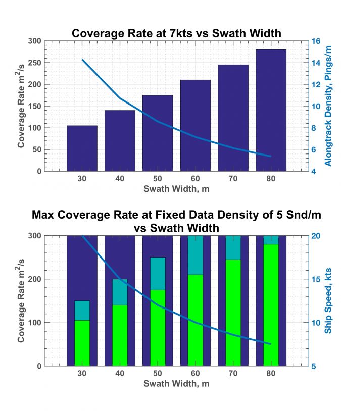
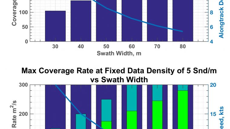
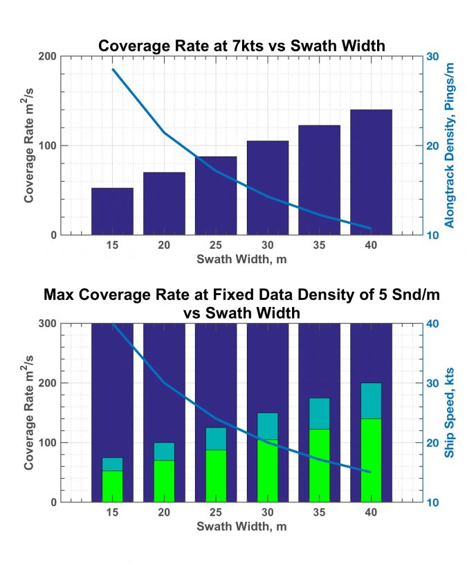
Consider Figure 1, in which the results of the model are illustrated for a survey in 10m of water under the two constraints of data density and survey speed. In Figure 1a, the ship’s speed is maintained at 7 knots and the coverage rate is shown in the bar plot as a function of swath width up to 8 x water depth (WD) (80m). As the swath width increases the coverage rate increases linearly from approximately 100 m^2/s at 30m swath width (3xWD), to 280 m^2/s at 80m swath width (8xWD).

Plotted on top of this bar graph in a blue line is the corresponding along-track ping spacing in pings per metre, which decreases from over 250 pings per metre at 30m swath width to just above 5 pings per metre at 80m swath width. Under these conditions of 10m nominal water depth, a low uncertainty sonar and benign refraction conditions, real survey efficiency gains can be achieved by increasing the swath width while maintaining the required data density.

Now consider Figure 1b, in which the along-track ping spacing is fixed to 5 pings per metre and the ship’s speed is varied to achieve this data density as the swath width increases. The navy bars indicating a constant, 300 m^2/s coverage rate with increasing swath width, show the effect alluded to above, in which the potential gains achieved by increasing the swath width are exactly offset by the need to decrease the vessel’s speed to maintain the 5 pings per metre data density.

Plotted atop the bar graph, as a blue line, is the vessel’s speed required to maintain the 5 pings per metre data density. The vessel’s speed is seen to decrease with the increase in swath width to accommodate the decreasing ping rate required of a wider swath. But note that at a 30m swath width, the vessel must go 20 knots to achieve this maximum theoretical coverage rate! A survey speed of this magnitude is, of course, impractical. As the swath width decreases, the vessel simply cannot go fast enough to maintain the maximum theoretical coverage rate.

Also in Figure 1b, plotted in cyan and green, are bars showing the coverage rate when vessel’s speed is limited to a more reasonable 7 knots and 10 knots, respectively, while maintaining the data density requirement at each swath width. Figures 1a and b illustrate that in 10m of water, under the combined constraints of 5 soundings per metre and practical survey speeds of 7-10 knots, a wider swath width indeed contributes directly to increased coverage rate!

One may rerun the model at nominal water depths of 5m and 20m. These results are shown in Figures 2a and b and 3a and b, respectively. In 5 metres of water, ping rates achievable at all swath widths considered are so high that meeting the along-track data density requirement is never a constraint for vessel speeds below 10 knots. Therefore, the wider the swath width (and faster the vessel) the greater the coverage rate.

In 20m of water, however, the results are different, and possibly unexpected. In 20m of water, the two-way travel time is relatively long, requiring relative low ping rates and slow vessel speeds to achieve the required along-track data density. For example, Figure 3a, which shows the coverage rate and along-track data density vs swath width at a fixed, 7 knots, survey speed shows that a swath width wider than 80m (4xWD) cannot achieve 5 pings per metre data density while maintaining 7 knots.

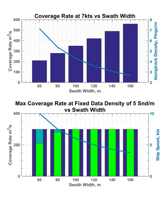
The effect is also seen in Figure 3b, in which the bars illustrating coverage rate when the data density is fixed at 5 pings per metre for various survey speeds are constant at all swath widths greater than 80m. The effect is largely the same for unrestrained speeds (blue bars), or when restrained to no more than 7 knots (cyan bars) or 10 knots (green bars). Therefore, efforts to increase swath beyond 3-4x water depth will require a reduction in survey speed to meet the data density requirement, exactly offsetting the effect of an increased swath width. When surveying in water depths greater than 20m, efforts to increase the swath beyond 3-4x water depth are fruitless.

No accommodation was given in the model to systems that can transmit multiple pings simultaneously. However, one can surmise the impact these systems can have from Figure 3a. Since the along-track data density is directly proportional to the ping rate, a doubling of the ping rate produces a doubling of the data density. While a single-ping system is limited to 3-4xWD to achieve 5 pings per metre, a doubling of the ping rate can produce a swath as much as 8xWD while maintaining the same 5 pings per metre constraint. Moreover, while increasing the swath width has no advantage in water deeper than 20m for a single ping system, it remains advantageous to increase the swath width in water as deep as 40m for a dual-ping system.

Conclusion - When to Maximise Swath Width

In summary, one may draw a few conclusions, as rules of thumb, from the models presented. When surveying in water depths deeper than about 20m, there is no advantage to increased swath width beyond 3-4xWD. A single-head multibeam echo sounder should suffice. However, when surveying in water shallower than 20m, particularly in depths 10m or less, strive to achieve the widest swath width possible, subject to meeting IHO uncertainty requirements and refraction conditions. Dual-head multibeam echo sounders or bathymetric side-scans, whose geometry lends itself to a wider swath width, can provide real coverage efficiency gains in these operations.