Shallow Survey 2005 Common Dataset Comparisons
Shallow Survey 2005 Common Dataset Comparisons As part of the Shallow Survey Conference 2005 held in Plymouth, swath sonar manufacturers were invited to survey a common dataset. Two regions were chosen: an offshore area south of Plymouth breakwater suited to larger vessels and Lidar operations, and an inshore area around Plymouth Hoe. The data collected for the inshore area serves as the basis for this study. The manufacturers and systems that provided data for the inshore area are listed in Table 1.
Each of the surveys was undertaken with the same supporting equipment, and mostly using the same vessel. RTK GPS, or similar, was used for positioning, and Applanix PosMV was used as a motion sensor and for position aiding. Each manufacturer was supplied with a technical specification outlining the survey requirements. They were all allowed five days to complete both the inshore and offshore survey areas. All manufacturer surveys took place during the summer of 2004. GeoAcoustics noticed some fundamental problems with their transducer and SV probe during processing of the initial survey data. They resurveyed both areas completely during the first week of June 2005. Only the 2005 data is included in the common dataset.
The inshore area was also surveyed using the ‘Aquaticsonar - Swathe Surveyor’ system. At the manufacturer’s request, the data from this system was not included in this comparison. The data was analysed but many of the features shown with the other systems were not present. The manufacturers’ reasons for this are published alongside this paper. The Aquaticsonar data is available in the Shallow Survey 2005 common data-set. Elac Nautik also requested withdrawal from the comparison, citing unfavourable weather during their survey period. The Elac Nautik data is available in the Shallow Survey 2005 common dataset.
Areas for Comparison
In order to provide a suitable comparison between the datasets, four specific areas were chosen within the inshore area that would hopefully highlight the capabilities of the systems (Figure 1).
Area 1:
To test each system’s capability to detect a 2m object (with reference to IHO order 1 specification and Land Information New Zealand Hyspec), a 2m cube manufactured from a steel frame with fibreglass sides was placed on the seabed in approximately 30m of water. This area (approximately 50m x 50m) covers the location of the 2m cube and also encompasses a small wreck in the south-east of the area. The loca-tion of the cube was unknown to the manufacturers at the time of data acquisition.
Area 2:
This area (approximately 100m x 100m) includes a rocky ridge with some near- vertical slopes and a sandy bottom. Swath systems often find bottom tracking difficult in these condtions, so this area was chosen to high- light such pos- sible problems.
The depth range is from 5m to 30m.
Area 3:
This area (approximately 25mx35m) contains what look like manmade linear objects, (17mx0.5m) 6m proud of the sea-bed, in approximately 14m of water. This area was chosen to show engineering-type applications of the systems.
Area 4:
An area (approximately 235m x 130m) of small sand waves in about 15m of water. This area was also chosen as it has a much softer bottom type than Area 2.
Comparing the Data
The data for the common dataset was supplied in various formats from the different manufacturers. The formats varied from full-density processed/ unprocessed, to gridded data. The highest-density datasets were always used, as some of the areas chosen for analysis required very small details to be seen, such as the objects in Area 3. In the case of unprocessed data, the UKHO had to undertake some basic processing, but this was only to remove obvious outliers and systematic errors. GeoAcoustics did not supply full-density data as part of the common dataset. For this study, GeoAccoustics supplied small areas of full-density data at the request of the UKHO. During the study a conscious effort was made to always provide an impartial comparison between the different datasets. The UKHO used Caris HIPS software throughout the study.
All plan-view images shown for each area have the same sun-illumination values and colour maps, e.g. 135º azimuth, 35º elevation for Area 1. The values were chosen to show the detail in all the datasets as clearly as possible, and not to show specific depth, as due to tidal errors this might not be the same for each survey. No vertical exaggeration or interpolation has been used in any of the plan views. The plan views also show the locations of any cross profiles (shown as black lines), taken as a slice (less than 1m wide) through the data points. Vertical exaggerations of 4 and 10 have been used in the various profile views.
For the beam-forming systems, shoal-bias surfaces are shown to highlight features. For the phase-measurement systems, mean surfaces are used, as these systems collect a much higher density of data and require the ‘mean grid’ of the data to ‘find’ the bottom depth. Figure 2 gives an example.
Points to note:
- The survey lines for each of the systems were not necessarily all run in the same direction.
- Not all of the areas were covered with the same density of data for each system, due to survey speed, swath widths and number of lines run in each area.
- The ping rates for each system were calculated using the actual time stamps of each ping in the data. The interferometric systems ping one side at a time; so six pings per second in the tables means 6 x port and 6 x starboard.
- The images shown here are Jpegs, and although they are good representations of the gridded data they cannot compare with full screen images from Caris HIPS software.
Area 1: The 2m Cube
The images in Figure 3 show the 2m cube in the top left, and the wreck (15m x 5m) in the bottom right. The black square outlines the Area 1 boundary. All images are from full-density datasets. The results are also visible in Table 2.
Area 2: Steep Ridge
All images of Area 2 are from full-density datasets. The cross profiles are all in the same location, as indicated on the plan-view images (Figures 4 and 5).
Of the four systems remaining in the trial, the SwathPlus also has the lowest data density in this area. The system shows a loss in slope definition near the bottom of the ridge. The GeoSwath has slightly noisy data but defines the slope well. The EM3002 shows a possible bottom-tracking problem, as seen in the profile view. See also Table 3 for results.
Area 3: Linear Objects
All images of Area 3 (Figure 6) are created from full-density datasets. Table 4 reflects the score for all products in the trial.
The datasets were binned at 0.2m to try and show the maximum definition possible. For most of the systems, in this depth of water this bin size is actually smaller than footprint size and would not necessarily be used for survey data. A 1.5° system would have a footprint of approximately 0.36m in 14m at NaDir compared with the 0.13m footprint of a 0.5° system. The 8125 system is able to obtain very high definition due to its 0.5° beam width. The GeoSwath system obtains very good data over the linear structures and is able to define them nearly as well as the 8125. For one of the two lines the GeoSwath system was configured to ping only on one side, so as to double the ping rate.
Area 4: Sand waves
All images shown in Figures 7, 8, 9 and 10 are from full-density datasets. The EM3002 system did not survey the entire area.
All of the systems manage to define the small sand waves, as seen in the cross profiles. The SwathPlus and GeoSwath do show noisier data in the cross profiles, though they are still able to define the sand waves, as shown in the gridded mean image. See also Table 5.
Overall Comments
The SwathPlus system has comparably lower data density than some of the other systems. This is apparent in the plan-view image of Area 2. Over the four areas the SwathPlus system generally had the widest swath width, lowest ping rates and highest vessel speeds. The combination of all these factors contributed to the lower data densities.
Conclusions
Area 1:
- All of the datasets show points recorded on the 2m cube, and in this example would all have passed the LINZ Hyspec v3 criteria for object detection.
- The wreck is visible in all of the datasets. The Reson SeaBat 8125 dataset appears to offer the clearest resolution of the wreck.
Area 2:
- All of the systems functioned well on the steep slope, the only issues being the low data densities of the SwathPlus system, and a possible side-lobe artefact visible in the EM3002 profile.
Area 3:
- The height of the objects above the seabed was found to be similar by all of the systems.
- The Reson SeaBat 8125 and Geo-Swath datasets offer the clearest resolution of the objects
- The EM3002 data lacks the definition of some of the other systems, considering the ping rate of the system in the area. The data is missing three of the linear structures in the bottom half of the plan-view image. This is possibly a bottom-tracking problem, as the structure stands proud of the seabed and may be treated as water-column noise due to a stronger return from the seabed.
Area 4:
- All of the datasets show the small 30cm high sand waves, though the EM3002 data shows them at the clearest resolution.
- None of the systems had problems tracking the soft sandy seabed.
There are still qualities of the data that would merit further analysis: backscatter, standard deviation, IHO-order compliance and 3D images. These issues will hopefully be included in a future expanded paper, to be made available at www.hydro-international.com.
Further Reading
Details of how to acquire the Shallow Survey 2005 Common Dataset can be found at the Shallow Survey website: www.shallowsurvey.com
Disclaimer
The views and opinions expressed in this paper are the personal opinion of the author and do not necessarily reflect those of the UKHO or the UK Ministry of Defence.
Acknowledgements
This paper would not have been possible without the co-operation of the four manufacturers who agreed to take part in the trial, and all of the six manufacturers who contributed to the Common Dataset did so at their own considerable expense. Thanks also to all those involved in the collection of the data:
Duncan Mallace at Netsurvey, Rick Read and various RN personnel at HMTG HMS Drake, and the Shallow Survey 2005 team.

Value staying current with hydrography?
Stay on the map with our expertly curated newsletters.
We provide educational insights, industry updates, and inspiring stories from the world of hydrography to help you learn, grow, and navigate your field with confidence. Don't miss out - subscribe today and ensure you're always informed, educated, and inspired by the latest in hydrographic technology and research.
Choose your newsletter(s)