INS and DVL for Out-of-Straightness Surveying
Inertial and Doppler, the Perfect Combination for 3D Pipeline Buckle Surveys
The move to deeper water, the proliferation of subsea completions, and the continued drive to lower costs are driving the requirement for more accurate out-of-straightness surveys. Pipelines are being designed to higher tolerances and are carrying warmer products at higher pressure. It is assumed that pipes will expand and move throughout their lifetime. Surveys are required to confirm that there are no un-planned buckles in the line. This article shows how INS (Inertial Navigation System) and DVL (Doppler Velocity Log) may be combined to meet these requirements.
Out-of-straightness surveys are required to confirm that the pipe has moved as expected and that there are no un-planned movements or buckles in the line. Typical requirements for an out-of-straightness survey are:
1. To be able to detect a deviation (XY&Z) from straight of +/-10cm over 100m length.
2. Repeatability of absolute position better than +/- 2m.
Previously, out-of-straightness surveys were conducted using USBL (Ultra-short Basline), DVL, and Pressure sensors. The USBL and DVL can be combined to produce a reasonably smooth track, but in deep water, accuracy is a problem. The Z component can be a major problem with this technique as the effect of swell on the pressure sensor can be significant even at relatively deep depths.
For out-of-straightness surveying work, an ROV is typically equipped with an INS closely coupled to a DVL, Pressure Sensor, Sound velocity sensor, GPS (when on deck) and USBL (when submerged). Experience has shown us that the best performance is obtained when the DVL is mounted rigidly to the INS. This configuration enables calibration of the misalignment between INS and DVL prior to installation on the ROV. Some customers prefer to mount the DVL and the INS side by side in order to save height, but for the survey described in this article a ’PHINS/DVL Ready’ combination was pre-calibrated, with the DVL securely bolted to the bottom of the INS.
Introduction to Inertial Navigation
An inertial navigation system is a set of electronics and sensors that very accurately measures acceleration and rotation rate. By mathematically integrating the acceleration and rotation rate data velocity and direction may be derived. Velocity and direction data may be combined with an initial starting position to calculate subsequent positions. No sensor is perfect and errors will always creep in to an inertial solution. Bias and scale factor errors accumulate over time leading to a drift in the calculated position. The INS (PHINS) used with no aiding sensors has a free inertial drift rate (no external aiding) of 0.6 nautical miles in 1 hour. A Kalman filter is implemented within the INS to take external aiding data and fuse that data with the inertial measurements. A large buffer within the Kalman filter allows the use of old data within the position calculation so-long as the age of that data is known.
GPS and USBL are both systems used to aid INS, they are both similar in character in that over a long period of time they are very accurate, they effectively have no drift rate. Over short periods of time they can be inaccurate with noise or spikes on the provided position.
The combination of inertial measurements with external position updates produces a positioning solution that has the best benefits from each system, High Update rate, Smooth, No Drift, Robust to drop outs, etc.
DVL is also used to aid INS. Combined with inertial measurements it will produce an even smoother position than USBL or GPS aiding but will produce a small position drift of typically 0.1% of travelled distance due to residual heading and speed errors. This article shows that combining USBL and DVL in post-processing will give the best smoothing and absolute position accuracy.
The rule of thumb for combining position aiding sensors with an iXBlue INS is that the real-time position noise is reduced by at least 3 times. Through the use of post-processing software, much better results may be achieved.
The Data Set
This data set made available to iXBlue consists only of the post-processing data logged from the INS, covering approximately 1.7km of pipeline survey. Approximately 1km down the pipeline is a designed curve, deviating 8 degrees over 300 metres.
In this case, the ROV was positioned using a USBL system and position updates were provided to the INS through the ROV umbilical and multiplexor. The ROV was fitted with an undercarriage and was driven along the top of the pipe in direct contact. In this way, by adding a simple leaver arm to the INS, the position of the top of the pipe can be directly measured by the inertial navigation system. A post-processing data stream which includes all the raw sensor and aiding data was logged to file and was used as the basis for this analysis. Because the data set is a complete record of the measurements the INS makes along with all the aiding data applied, complete re-processing of the data is possible.
IXSEA INS post-processing software DelphINS was used to re-process the logged data. Extensive re-processing is possible, correcting settings, changing offsets etc, even changing the standard deviation of input data and hence modifying how the algorithm treats that data is possible. The software uses the same algorithm as is used in the INS during real-time operations. Multiple processing techniques were used and are discussed here.
To calculate ’out-of-straightness’, a text format file was output from DelphINS at a rate of one position per second, for each point in this track the point 50m either side of the point of interest is calculated. Next, the best fit line through this data is calculated using a linear least squares technique. This results in a straight line that best fits the 100m section around each point on the track. The out-of-straightness figure produced for each point is the lateral distance to each best fit line.
Problems with USBL Data
Although most USBL systems claim accuracy of 0.2% slant range, real world data rarely achieves these levels of accuracy; specifications are only valid for certain environmental conditions which are rarely met in field operations. In addition, the total error budget for the USBL system cannot be taken in isolation, but also involves the motion sensor, gyrocompass, leaver arms, mounting flex and GPS accuracy.
In Figure 2, we can see the USBL data contains a number of obvious spikes. For some reason, in this data set, the spikes to the North are much larger but less numerous than the spikes to the south of the track. We can also see that the trend of the USBL data is not entirely linear when compared with the best fit line for this section of data.
The noise and spikes on the USBL data rule it out for OOS purposes, but there are additional problems with the USBL data that adversely affect the real-time INS track (blue). In this case, the USBL data being provided to the PHINS included unrealistic estimations of standard deviation. In some cases, where the spikes occur, the supplied position SD is dropping very low. Effectively, the PHINS is being told that this USBL data is unrealistically accurate; this causes the INS to follow the USBL data far more than it should.
Effects of Poor Aiding Data
To fully understand why the real-time data is not better than this it is important to understand how the PHINS uses external data.
iXBlue INS systems all process external data based on the reported standard deviation of that data. Where no standard deviation is explicitly specified by the input protocol, a default is used based on the type of data, GPS, USBL, LBL, DVL etc. These default values have been chosen such that a workable INS track will be produced in any circumstances i.e. they are a compromise. Imagine a surface vessel with a DVL mounted on an over the side pole, working at extreme range and a lot of vessel motion. Compare that situation to an OOS survey, with a high frequency DVL on a stable platform close to the seabed. The default settings must produce useful results in both of these circumstances.
The INS checks input data for consistency with its own internal estimation of position and an associated standard deviation, the PHINS compares its own internal position plus standard deviation with the externally supplied aiding position plus standard deviation, if there is overlap between the two positions plus standard deviations, then the aiding data is considered valid. If there is no overlap the data is rejected and not applied to the Kalman filter. This means that by using a small standard deviation on the input data spikes will be rejected, however, the smaller the standard deviation, the more emphasis INS puts on that data and therefore small noise in the data will have more effect on the INS position.
Optimal Processing
By de-spiking the USBL data, tuning the standard deviation for both the USBL and the DVL, we can re-process the complete pipeline survey to produce positioning data suitable for ’As Laid’ chart production. The inclusion of USBL data means the position is drift free, and the tuning of the standard deviations produces a track that is smooth and relatively accurate, but still influenced slightly by USBL noise, notably by any residual biases.
In order to produce a track suitable for Out-of-Straightness analysis, the USBL must be discarded entirely. With no DVL the drift will exceed the specifications mentioned earlier in a matter of seconds, speed errors build up because of bias on the accelerometers. The INS has no way to detect nor correct these errors. DVL data allows the INS to correct these speed errors by providing a speed update which can be used to estimate the bias errors.
Conclusion
Using DelphINS software to reprocess the data with the USBL disabled results in a track with a drift rate of 0.1% distance travelled, 1.7m over the length of this track or 10cm over 100m. This meets the required accuracy specifications so long as the processed track is less than 2km, ample to cover most areas of interest for out-of-straightness analysis. Figure 3 shows the results of the OOS processing, both on the optimal processed track and on the original real-time track. Figure 4 shows an example of the effect of the optimal processing on a Multi-beam based Out-of-Straightness survey.

Value staying current with hydrography?
Stay on the map with our expertly curated newsletters.
We provide educational insights, industry updates, and inspiring stories from the world of hydrography to help you learn, grow, and navigate your field with confidence. Don't miss out - subscribe today and ensure you're always informed, educated, and inspired by the latest in hydrographic technology and research.
Choose your newsletter(s)